Lab 0: Prerequisite Material
Functions
- Function—a rule, usually denoted by a single letter, say f, that assigns to each element x in a set D exactly one element, called f(x), in a set R.
In calculus, both the sets D and R are subsets of the real numbers.
- Domain—the set D is often referred to as the domain of the function. When you are asked to find the domain of a function, you will look for x-values for which the function is defined.
- Range—the set, R, of all values of f(x) as x varies throughout its domain, D.
Functions can be described in four different ways.
- Verbally
"Take each real number times itself."
-
Numerically
x −2 −1 0 1 1.5 2 e 3 \pi f(x) 4 1 0 1 2.25 4 e2 9 \pi2 - Visually
- Algebraically
f(x) = x^2
In calculus, you need to be able to work with functions in all four forms, but you will most frequently work with the algebraic form. Knowing the graphical form of various functions will be helpful to you throughout calculus.
When dealing with any expression, you need to be able to determine whether or not the expression is a function. You need to understand the definition of a function to make this determination. A layperson's definition of a function might be "for each x-value, there is one and only one y-value." The first example below is a function and the second one is not. Can you explain why (in both cases)?
Example 0.1:
F| x | −2 | −1.5 | −1 | 0 | 1 | 2 | 3 |
|---|---|---|---|---|---|---|---|
| y | 5 | 4 | 2 | 1 | 4 | 3 | 5 |
Even though we have y-values that are the same, each of these y-values is associated with two different x-values so F is a function.
Example 0.2:
G| x | −3 | −2 | −1 | −1 | 0 | 1 | 2 |
|---|---|---|---|---|---|---|---|
| y | −1 | −5 | 4 | 3 | 2 | 3 | 7 |
Here we have the same x-values being mapped to two different y-values so G is not a function.
One advantage of the graphical representation of an expression is that it makes it easy to determine whether or not an expression is a function of x because you can use the vertical line test.
- The Vertical Line Test—A graph in the xy-plane is the graph of y as a function of x if and only if any vertical line intersects the graph at most once.
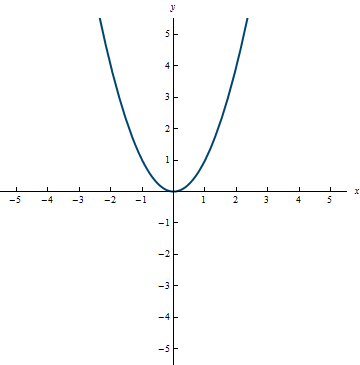
Example 0.3:
Function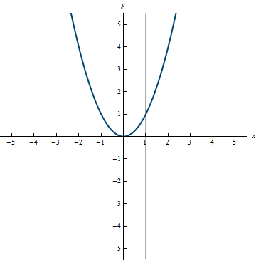
In the graph above, you can see that no matter where a vertical line is drawn, it will never intersect the curve more than once.
Example 0.4:
Not a function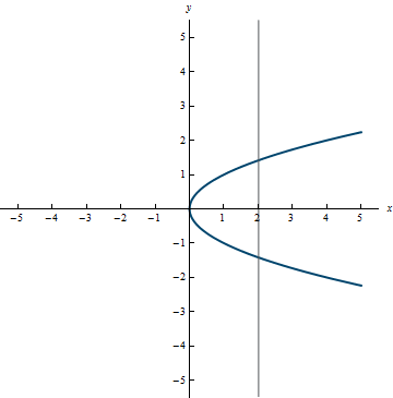
In this graph, you can see that the vertical line x = 2 will intersect the curve twice.
Different Kinds of Functions
There are numerous kinds of functions that you will encounter in calculus. The ones included in this section are ones that you should know how to graph and you should know characteristics of them. A highlighted label indicates that the example is a graph you should memorize, because the example is used frequently in calculus.
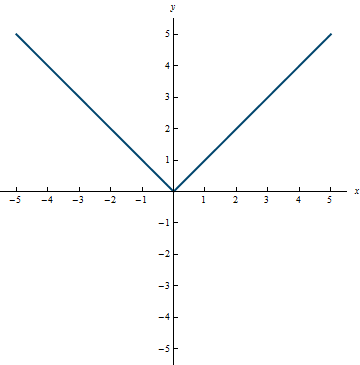
- Piecewise defined function—a function whose definition is different for different portions of its domain.
Example 0.5

Range: (-\infty, 0] \cup (2, \infty)
Example 0.6
Range: [0, \infty)
- Polynomial function—the general form of a polynomial of degree n is P(x) = a_nx^n + a_{n - 1}x^{n - 1} \;+ \, ... \, +\; a_1x + a_0, where a_n \ne 0.
A polynomial of degree 0 is called a constant function and its graph is a horizontal line with equation, y = c, where c is the constant y-value where the graph crosses the y-axis.
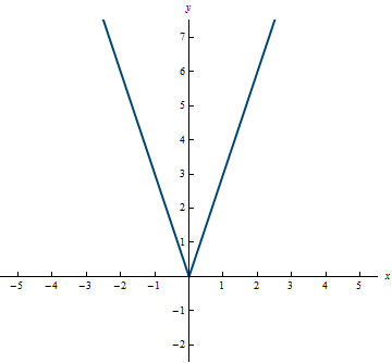
A polynomial of degree 1 is called a linear function, with equation given by y = f(x) = mx + b, where m \ne 0.
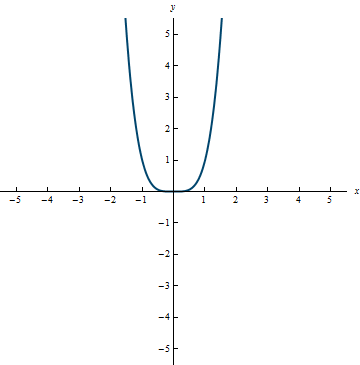
A polynomial of degree 2 is called a quadratic function, with equation given by f(x) = ax^2 + bx + c, where a \ne 0.
A polynomial of degree 3 is called a cubic function.
A polynomial of degree 4 is called a quartic function.
Some special polynomials that you should know well are graphed in the following examples.
Example 0.7
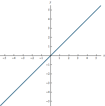
Range: (-\infty, \infty)
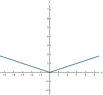
Example 0.8

Range: [0, \infty)
Example 0.9
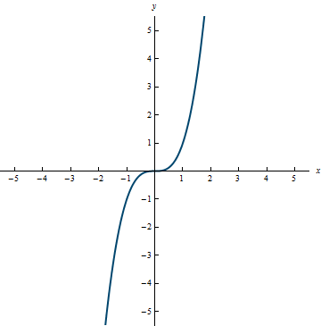
Range: (-\infty, \infty)
Example 0.10
Range: [0, \infty)
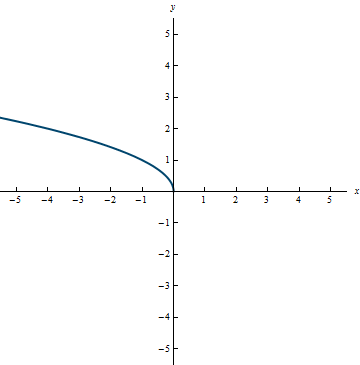
- Root function—a root function is a function of the form y = f(x) = \sqrt[n]{x} = x^{1/n}, where n is a positive integer.
When finding the domain of the root function, you should be careful. In calculus, we will be working with real numbers and since an even root of a negative number yields a complex number, the domain for the root function when n is a positive even integer will be [0, \infty).
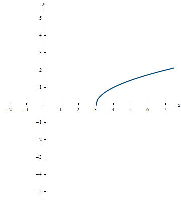
Example 0.11
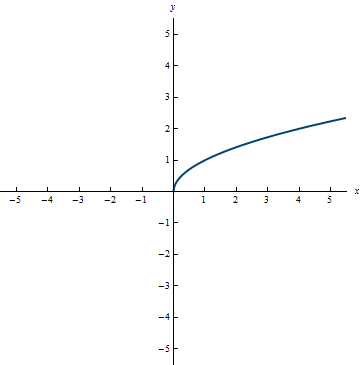
Range: [0, \infty)
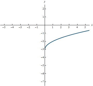
Example 0.12
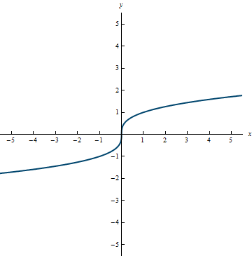
Range: (-\infty, \infty)
- Rational function—a rational function is a ratio of two polynomials, f(x) = \frac{P(x)}{Q(x)}.
You need to be careful when finding the domain of rational functions. Be sure that you exclude from the domain x-values that would make Q(x) = 0. In addition, you want to be careful about x-values that make both P(x) = 0 and Q(x) = 0 as this results in the indeterminate form, \frac{0}{0}.
Example 0.13
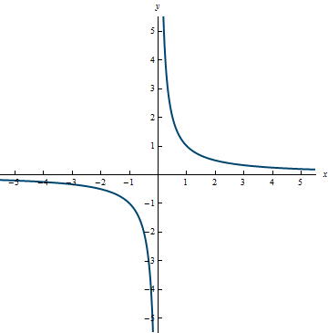
Range: (-\infty, 0) \cup (0, \infty)
Example 0.14
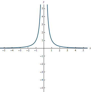
Range: (0, \infty)
- Algebraic function—An algebraic function is a function that is created using a finite number of algebraic operations (such as addition, subtraction, multiplication, division, and taking roots). Polynomials, root functions, and rational functions that have already been mentioned are examples of algebraic functions. Some algebraic functions are more complicated, such as f(x) = x^3\sqrt{x^2 - 6x + 3} or g(x) = \dfrac{x^2 - 5x^4}{\sqrt{x} - x}.
- Transcendental Functions—Transcendental functions are functions that are not algebraic. Although it is not easy to show, examples of transcendental functions include the trigonometric functions, exponential functions, logarithmic functions, and inverse trig functions (which we will explore in detail later).
Transformations of Functions
Now that we have encountered various types of functions, let's discuss how we can transform functions. Understanding these transformations and knowing the graphs that you have seen so far, you should be able to graph lots of functions very quickly.
- Vertical and Horizontal Shifts. Suppose b > 0. The graph of:
- y = g(x) + b means shifting the graph of y = g(x) b units up.
- y = g(x) - b means shifting the graph of y = g(x) b units down.
- y = g(x - b) means shifting the graph of y = g(x) b units to the right.
- y = g(x + b) means shifting the graph of y = g(x) b units to the left.
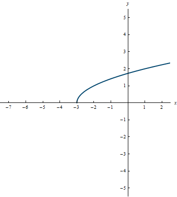
Example 0.15
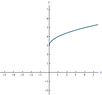
Example 0.16
Example 0.17
Example 0.18
- Reflections. The graph of:
- y = -g(x) means reflecting the graph of y = g(x) about the x-axis.
- y = g(-x) means reflecting the graph of y = f(x) about the y-axis.
Example 0.19
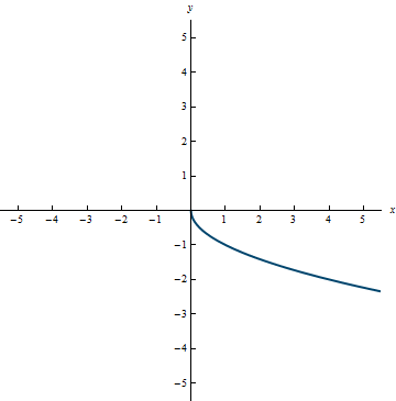
Example 0.20
- Vertical and Horizontal Stretching and Compressing. Suppose b > 1. The graph of:
- y = bg(x) means stretching the graph of y = g(x) vertically by a factor of b.
- y = \frac{1}{b}g(x) means compressing the graph of y = g(x) vertically by a factor of b.
- y = g(bx) means compressing the graph of y = g(x) horizontally by a factor of b.
- y = g\left(\frac{1}{b}x\right) means stretching the graph of y = g(x) horizontally by a factor of b.
Example 0.21
Example 0.22
Combinations of Functions
We have already briefly discussed combining functions, using the composition of functions. We will discuss composition again as well as other operations that can be used to combine functions.
Two functions f and g can be combined to form new functions in a manner similar to the way we add, subtract, multiply, and divide real numbers.
- (f + g)(x) = f(x) + g(x)
- (f - g)(x) = f(x) - g(x)
- (fg)(x) = f(x) \cdot g(x)
- \left(\frac{f}{g}\right)(x) = \frac{f(x)}{g(x)}, g(x) \ne 0
Basic Trigonometric Review
Trigonometry is an essential part of the study of calculus. A good trigonometry background is essential for you as a student of calculus. This section will focus on some concepts from trigonometry that you need to know in order for you to be successful in the calculus sequence. Do not think of this section as a series of facts to memorize but rather information that you need to learn and understand.
- Right Triangle Trigonometry
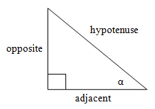
Given a right triangle, we can define the six trigonometric functions for an acute angle in the triangle, using the sides of the right triangle. We will also use some abbreviations: the abbreviation for sine is sin, the abbreviation for cosine is cos, the abbreviation for tangent is tan, the abbreviation for cosecant is csc, the abbreviation for secant is sec, and the abbreviation for cotangent is cot. A picture of the scenario will be helpful (see Figure 0.1). We will call our acute angle \alpha and label the side of the triangle adjacent to \alpha as adjacent, the side opposite \alpha as opposite, and the longest side opposite the right angle as the hypotenuse. Now we can define the six trigonometric functions for \alpha using the ratios of these sides.
Figure 0.1
 \begin{array}{rclcrcl}
\sin(\alpha) & = & \frac{\text{opposite}}{\text{hypotenuse}} &&& \\
\cos(\alpha) & = & \frac{\text{adjacent}}{\text{hypotenuse}} &&& \\
\tan(\alpha) & = & \frac{\text{opposite}}{\text{adjacent}} & \implies & \tan(\alpha) & = & \frac{\sin(\alpha)}{\cos(\alpha)} \\
\csc(\alpha) & = & \frac{\text{hypotenuse}}{\text{opposite}} & \implies & \csc(\alpha) & = & \frac{1}{\sin(\alpha)} \\
\sec(\alpha) & = & \frac{\text{hypotenuse}}{\text{adjacent}} & \implies & \sec(\alpha) & = & \frac{1}{\cos(\alpha)} \\
\cot(\alpha) & = & \frac{\text{adjacent}}{\text{opposite}} & \implies & \cot(\alpha) & = & \frac{1}{\tan(\alpha)}
\end{array}
\begin{array}{rclcrcl}
\sin(\alpha) & = & \frac{\text{opposite}}{\text{hypotenuse}} &&& \\
\cos(\alpha) & = & \frac{\text{adjacent}}{\text{hypotenuse}} &&& \\
\tan(\alpha) & = & \frac{\text{opposite}}{\text{adjacent}} & \implies & \tan(\alpha) & = & \frac{\sin(\alpha)}{\cos(\alpha)} \\
\csc(\alpha) & = & \frac{\text{hypotenuse}}{\text{opposite}} & \implies & \csc(\alpha) & = & \frac{1}{\sin(\alpha)} \\
\sec(\alpha) & = & \frac{\text{hypotenuse}}{\text{adjacent}} & \implies & \sec(\alpha) & = & \frac{1}{\cos(\alpha)} \\
\cot(\alpha) & = & \frac{\text{adjacent}}{\text{opposite}} & \implies & \cot(\alpha) & = & \frac{1}{\tan(\alpha)}
\end{array}
The Unit Circle
You need to know the values of all six trigonometric functions at any of the special angles on the unit circle. The special angles include all multiples of \frac{\pi}{6} \; (30^{\circ}), all multiples of \frac{\pi}{4} \; (45^{\circ}), all multiples of \frac{\pi}{3} \; (60^{\circ}), all multiples of \frac{\pi}{2} \; (90^{\circ}), and all multiples of \pi \; (180^{\circ}). If you can learn these values for the angles in quadrant I, then you should be able to translate this knowledge to any of the important angles in the other quadrants. Essentially, you need to know the Pythagorean Theorem, some geometry, and remember that you are using a unit circle (circle of radius 1). I credit the explanations that follow for cosine and sine to my colleague and friend, Dr. Christine Larson.
Most of you are more comfortable using degree measure for angles, but in calculus we always use radian measure. Now is a good time to review how to convert between the two angle measures. Hopefully you remember that 180^{\circ} = \pi radians. If you are given an angle in degrees and you want to convert it to radians, you will need to multiply the angle by \frac{\pi \text{ radians}}{180^{\circ}}. If you are given an angle in radians and want to convert it to degrees, you need to multiply the angle by \frac{180^{\circ}}{\pi \text{ radians}}.
- Thorough Explanation for Cosine and Sine of \frac{\pi}{4}
Figure 0.2
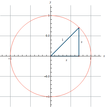
Looking at Figure 0.2, you see a right isosceles triangle in the first quadrant of the unit circle (circle with radius 1). In fact, we have a 45-45-90 triangle. Using the Pythagorean Theorem, we get the equation x^2 + x^2 = 1^2. Solving this equation for x yields x = \pm \frac{1}{\sqrt{2}} and since the point is in the quadrant I, we know that x must be positive. So, we have that the length of each leg of this right triangle is \frac{1}{\sqrt{2}} or \frac{\sqrt{2}}{2}. The coordinates of the point on the circle are \left(\frac{1}{\sqrt{2}}, \frac{1}{\sqrt{2}}\right). When using the unit circle, the cosine of the angle between the hypotenuse and the positive x-axis is given by the x-coordinate and the sine of the angle is given by the y-coordinate. In calculus, we always use radians instead of degrees so we have that \cos\left(\frac{\pi}{4}\right) = \frac{1}{\sqrt{2}} and \sin\left(\frac{\pi}{4}\right) = \frac{1}{\sqrt{2}}.
Understanding this information, using reference angles, and knowing the algebraic sign of x and y in all of the quadrants allows us to know the values of the trigonometric functions for the following angles on the unit circle: \frac{3\pi}{4}, \frac{5\pi}{4}, and \frac{7\pi}{4}.
- Thorough Explanation for Cosine and Sine of \frac{\pi}{6} and \frac{\pi}{3}
Figure 0.3
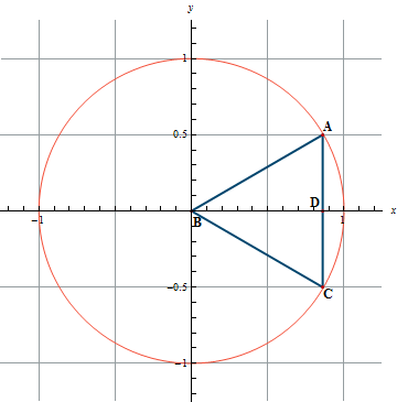
The triangle ACB was constructed as an equilateral triangle. Since BA and BC are radii of the unit circle, they have a length of one unit. Thus, the length of AC will also be one unit. From geometry, we know that an equilateral triangle is also equiangular so the measures of the angles at A, C, and B are all 60 degrees or \frac{\pi}{3} radians. BD was constructed as the perpendicular bisector of AC, and we know from geometry that it will also be the angle bisector for angle B. Thus, we have that triangle BAD is a 30-60-90 triangle with BA = 1, and AD = \frac{1}{2} so by the Pythagorean Theorem we can solve for BD.
BD^2 + \left(\frac{1}{2}\right)^2 = 1^2 will give us that BD = \pm\frac{\sqrt{3}}{2}, but since BD is a length on the positive x-axis, we have that BD = \frac{\sqrt{3}}{2}. Now, we have the coordinates of the point A and they are \left(\frac{\sqrt{3}}{2}, \frac{1}{2}\right). Since the x-coordinate represents the cosine of ∠ABD and the y-coordinate represents the sine of ∠ABD, we have that \cos\left(\frac{\pi}{6}\right) = \frac{\sqrt{3}}{2} and \sin\left(\frac{\pi}{6}\right) = \frac{1}{2}. Now you might be wondering why it is \frac{\pi}{6} instead of \frac{\pi}{3}, but remember that ∠ABC was \frac{\pi}{3} and BD is the angle bisector so ∠ABD will be half of the angle, \frac{\pi}{6}. In triangle ABD, the angle at A is 60 degrees or \frac{\pi}{3} radians and if we recall that the cosine of an angle in a right triangle is defined as \frac{\text{adjacent}}{\text{hypotenuse}} and that the sine of the angle in a right triangle is defined as \frac{\text{opposite}}{\text{hypotenuse}}, we can use these facts to find the cosine and sine of \frac{\pi}{3}. Using triangle ABD with angle A equal to \frac{\pi}{3} radians, we have that \cos\left(\frac{\pi}{3}\right) = \frac{\text{adjacent}}{\text{hypotenuse}} = \frac{1/2}{1} = \frac{1}{2} and \sin\left(\frac{\pi}{3}\right) = \frac{\text{opposite}}{\text{hypotenuse}} = \frac{\sqrt{3}/2}{1} = \frac{\sqrt{3}}{2}.
Understanding this information, using reference angles, and knowing the algebraic sign of x and y in all of the quadrants allows us to know the values of the trigonometric functions for the following angles on the unit circle: \frac{2\pi}{3}, \frac{5\pi}{6}, \frac{7\pi}{6}, \frac{4\pi}{3}, \frac{5\pi}{3}, and \frac{11\pi}{6}.