
Lab 7 - LR Circuits
Introduction
The English physicist Michael Faraday found in 1831 that when the current through a coil changes, the coil produces a changing magnetic field (in addition to the field of the changing current), which induces an electromotive force ("emf") in the coil itself. In 1834, the German physicist Heinrich Lenz refined this further by showing that the induced current driven by this emf will be in the direction that opposes the change in the original current. We call this phenomenon self-induction, and the coils are called inductors. At the time that Faraday announced his discovery, he was asked what possible use such knowledge could be? His reply was: "Of what use is a newborn baby?" As happens with many seemingly arcane discoveries, Faraday's investigations of induction led to several common and useful modern electrical devices. Inductors, like capacitors, affect the time characteristics of an AC (alternating current) circuit and are, therefore, used to tune radio circuits, filter out unwanted noise, etc. The telephone receiver makes use of a type of inductor, as do stereo speaker systems and microphones. In this lab you will examine the effect of an inductor on the current and voltage in a simple circuit.Discussion of Principles
The inductance of a circuit, usually symbolized by L, and measured in henry (H), is the tendency of a circuit to oppose any changes in the current. This opposition to a change in the current shows up as a slowing of the rise or fall of the current in circuits. Inductance is a property of electrical devices. Devices having this property are called inductors. The inductance of a device, like resistance and capacitance, depends on geometrical factors like the size of the device and on the material from which the device is made. It does not depend on the current in the device. Consider a simple circuit consisting of a switch, a resistor R, and a battery. When the switch is closed, the current I in the circuit will increase very quickly to a steady value given by Ohm's Law,I = ΔV / R,
where ΔV
is the voltage or emf of the battery. Consider the same circuit with the addition of an inductor, as shown in Fig. 1.
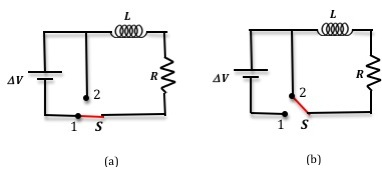
Figure 1: LR circuit
( 1 )
ΔV − IR − L
= 0.
| dI |
| dt |
ΔV − IR − L
= 0.
| dI |
| dt |
( 2 )
I = If
1 − e(−R/L)t
 |
 |
( 3 )
IR − L
= 0.
| dI |
| dt |
IR − L
= 0.
| dI |
| dt |
( 4 )
I = I0e(−R/L)t
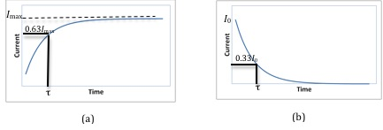
Figure 2: Current versus time graph
Time Constant
The mathematical analysis of a simple LR circuit is similar to that of a simple RC circuit (a circuit consisting of a resistor and a capacitor in series). In an RL circuit, the time constantτ
is defined by
( 5 )
τ = L/R.
(1 − e−1)
of its final value. Note that Eq. (2)I = If
1 − e(−R/L)t
has the same form as the equation describing the charging of a capacitor.
Since the current is changing with time, the potential difference across the resistor must also be changing with time. The equation for the potential difference across the resistor is obtained by using Ohm's Law, |
|
ΔV = IR,
( 6 )
ΔVR = ΔVf
1 − e(−t/τ)
|
|
ΔVf
is the final or maximum potential difference across the resistor and is equal to the emf of the battery.
Note that at t = 0, (1−e−t/τ) = 0
and the current through the circuit and the potential difference across the resistor are zero. Therefore, the potential drop is entirely across the inductor. At t = infinity (a long time after the switch has been in position 1), (1 − e−t/τ) = 1
and the current through the circuit and the potential difference across the resistor are maximum at If and ΔVR.
Therefore, the potential drop is entirely across the resistor and the potential drop across the inductor is zero.
Without the inductor in the circuit the current in the resistor would drop very quickly to zero once the switch is moved to position 2. When the inductor is in the circuit, it opposes this change in current, and so the current drops more slowly. The current and voltage across the resistor t seconds after the battery is removed from the circuit by moving the switch to position 2 are given by the following.
( 7 )
I = I0e(−t/τ)
( 8 )
ΔVR = ΔV0e(−t/τ)
τ
is the time needed for the current to decrease to 33% of its original value at t = 0.
Consider Eq. (7)I = I0e(−t/τ)
and Eq. (8)ΔVR = ΔV0e(−t/τ)
. At t = 0, e−t/τ = 1,
and the current through the circuit and the potential difference across the resistor are maximum. Therefore, the potential drop is entirely across the resistor and the potential drop across the inductor is zero. At t = infinity (a long time after the switch has been in position 2), e−t/τ = 0,
and the current through the circuit and the potential difference across the resistor are zero. Therefore, the potential drop is entirely across the inductor and the potential drop across the resistor is zero.
At any given time t the sum of the potential drops across the resistor and the inductor will be equal to the emf of the battery.
( 9 )
emfbattery = ΔVR + ΔVL
ΔVR
across the resistor as a function of time is shown here in Fig. 3 and Fig. 4 shows the voltage drop across the inductor as a function of time. Note that when the voltage across the resistor is a maximum, the voltage across the inductor is zero and vice versa as discussed earlier.
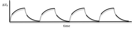
Figure 3: Voltage across the resistor as a function of time
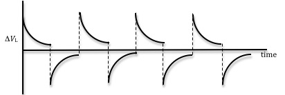
Figure 4: Voltage across the inductor as a function of time
ΔVR = ΔVf
1 − e(−t/τ)
can be algebraically rearranged as:
|
|
( 10 )
| ΔVf − ΔVR |
| ΔVf |
τ
has been replaced with L/R. Taking the natural log of both sides of this equation and multiplying by –1, we get
( 11 )
−ln
=
t.
 |
| ΔVf − ΔVR |
| ΔVf |
 |
| R |
| L |
y = (R/L)t,
which is a linear equation of the form y = mx.
The inductance can be determined from the slope of this line.
Similarly, Eq. (8)ΔVR = ΔV0e(−t/τ)
can be written as
( 12 )
−ln
=
t.
|
| ΔVR |
| ΔV0 |
|
| R |
| L |
−ln
versus time t for a decreasing current (soon after the switch is opened) will give a straight line with a slope of R/L from which the inductance can be determined.
|
| ΔVR |
| ΔV0 |
|
Using a Square Wave to Simulate the Role of a Switch
In this experiment, rather than using a switch, we will be using a signal generator that can generate periodic wave forms of varying shapes, like a sine wave, a triangular wave, and a square wave. Both the frequencies and amplitudes of the wave forms can also be adjusted. Here we will use the signal generator to produce a time-varying voltage, with a square wave form, across the inductor similar to the one shown in Fig. 5.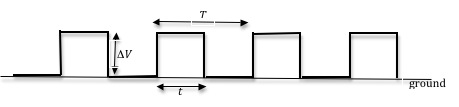
Figure 5: A square wave with period T
T = 2t
is the period of the square wave. During the first half of the cycle, when the voltage is positive, it is similar to the switch being in position 1. During the second half of the cycle, when the voltage is zero, it is the same as the switch being in position 2. So the square wave, which is a DC voltage that is turned on and off periodically, serves as both battery and switch in the setup in Fig. 1.
The signal generator allows this switching to be done repeatedly, and it is possible to optimize the data collection by adjusting the frequency of the repetition. This frequency will depend on the time constant of the RL circuit.
When the time t is larger than the time constant τ
of the RL circuit, the current in the circuit will have enough time to reach the steady state and the voltage across the inductor will be as shown in Fig. 4.
Objective
The objective of this experiment is to examine the dynamic behavior of an LR circuit by using an oscilloscope to visualize the voltage across the resistor for both rising and decreasing current. You will also determine the time constant and inductance of the coil.Equipment
- PASCO circuit board
- Capstone software
- Signal interface with power output
- Connecting wires
- Multimeter
Procedure
Please print the worksheet for this lab. You will need this sheet to record your data.
Setting Up the LR Circuit
The RLC circuit board that you will be using consists of three resistors and one inductance coil among other elements. The value of the inductor can be changed by inserting an iron core into the coil. See Fig. 6 below. In theory you can, therefore, have different combinations of resistors and capacitors. In this experiment you will use the 10-Ω resistor and the inductor coil.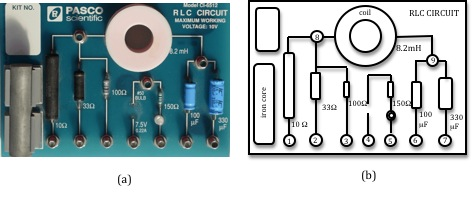
Figure 6: RLC circuit board
1
Connect the far right output terminal of the signal interface to the inductor at point 9.
2
Connect point 1 to the second output terminal of the signal interface to complete the circuit.
3
Connect the voltage probe into analog channel A.
4
To measure the voltage across the resistor, connect one lead of the voltage probe to point 8 and the other lead to point 1.
Make sure that the ground of the interface (the "–" lead) is connected to the same side of the resistor as the ground of the signal generator (power output).
Your circuit connection should look like that in Fig. 7.
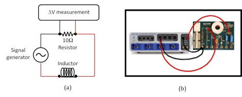
Figure 7: Circuit diagram
Checkpoint 1:
Ask your TA to check your connections before proceeding.
Ask your TA to check your connections before proceeding.
Procedure A: Determining L from Time Constant
The computer will function as the oscilloscope to recordΔVR
and as the signal generator.
5
Open the Capstone file associated with this lab. A screen similar to Fig. 8 is displayed.
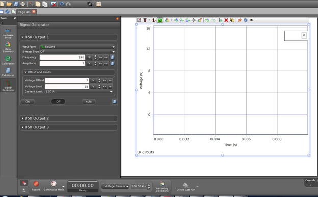
Figure 8: Opening screen of LR circuit file
6
The file should open with the signal generator set to produce a positive square wave.
7
If not already set, set the voltage to 7-V amplitude with the frequency at any value between 120 and 180 Hz and set the voltage offset to 7 V.
8
Turn on the signal generator by clicking ON in the signal generator window, and monitor the signal by clicking MONITOR in the main window. There should be a signal trace like that shown in Fig. 9. This will allow you to observe how the voltage on the resistor varies as a function of time. Click STOP after a few seconds. The data will remain in the scope window until the next time the START button is clicked.
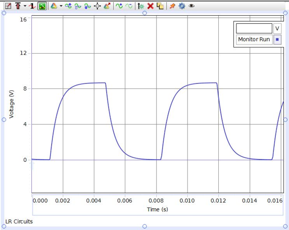
Figure 9: A sample signal
9
Adjust the voltage (potential difference) and time scales so that about one wavelength is displayed in the scope window, by placing the cursor on the values of each scale and dragging left-right or up-down as appropriate.
10
Select the Show Coordinates button from the buttons above the graph. See Fig. 10.
11
Using Show Coordinates, determine the starting time (i.e., when the potential difference begins to increase from 0 volts) and record it on the worksheet.
12
Calculate 63% of the maximum potential difference (0.63 ΔVf).
13
Use Show Coordinates to determine the time at which that potential difference occurs. Record this time on the worksheet.
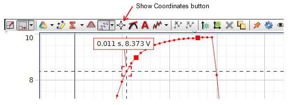
Figure 10: Show Coordinates
14
From the two time values obtained in steps 11 and 13, determine and record the time required for the signal to go from ΔVR = 0 to ΔVR = 0.63 ΔVf.
This is your experimental value for the time constant τ.
15
Use a multimeter to measure the combined resistance of the coil and resistor in series. This is the total resistance of the circuit. See Appendix K.
To do this, remove any other wire leads from the PASCO circuit board and then connect the multimeter around the resistor and inductor combination, as shown in Fig. 11.
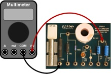
Figure 11: Physical wiring to measure total resistance of RL circuit
16
Calculate the experimental value of the inductance using Eq. (5)τ = L/R.
and the experimental values of τ
and R. Record this value on the worksheet.
17
Use the inductance value printed next to the inductor on the PASCO circuit board as the accepted value, and record this on the worksheet.
18
Calculate the percent error between the experimental and accepted values of the inductance, and record it on the worksheet. See Appendix B.
Checkpoint 2:
Ask your TA to check your data and calculations.
Ask your TA to check your data and calculations.
Procedure B: Measuring Voltage for Increasing Current
19
From the recorded oscilloscope trace, measure the voltage ΔVR
across the resistor and the time t for six points on the rising part of the curve. Record these values in Data Table 1.
20
From the final potential difference and the values of ΔVR
that you just recorded, calculate the quantities for the remaining two columns in Data Table 1.
21
Use Excel to plot −ln[(ΔVf − ΔVR)/ΔVf ]
versus t for the six points. See Appendix G.
22
Using the trendline option in Excel to draw the best fit line to your data, determine the slope of the line. See Appendix H. Record this on the worksheet.
23
Use the slope value to find the inductance and record this on the worksheet.
24
Calculate the percent error between the accepted value of the inductance and the value obtained from the slope of the graph. Record this value on the worksheet.
Checkpoint 3:
Ask your TA to check your data, Excel graph, and calculations.
Ask your TA to check your data, Excel graph, and calculations.
Procedure C: Measuring Voltage for Decreasing Current
25
From the recorded oscilloscope trace, measure the voltage ΔVR
across the resistor and the time t for six points on the falling part of the curve. Record these values in Data Table 2.
Note that ΔV0
for the falling part of the curve is the same as ΔVf
for the rising part of the curve.
26
From the initial potential difference ΔV0
and the values of ΔVR
that you just recorded, calculate the quantities for the remaining two columns in Data Table 2.
27
Use Excel to plot −ln[(ΔVR)/ΔV0]
versus t for your six points.
28
Using the trendline option in Excel to draw the best fit line to your data, determine the slope of the line and record this value on the worksheet.
29
From the slope value find the inductance and record this on the worksheet.
30
Calculate the percent error between the accepted value of the inductance and the value obtained from the slope of −ln[(ΔVR)/ΔV0]
versus t graph. Record this value on the worksheet.
Checkpoint 4:
Ask your TA to check your data, Excel graph, and calculations.
Ask your TA to check your data, Excel graph, and calculations.