Appendix H: Adding A Trendline to a Graph

As you might know, it is easy to create a chart of existing data using Excel. It is equally easy to add a trendline (line of best fit) to your data and display the equation to the trendline in Excel. From the equation to the trendline the slope and intercept can be determined.

1
To add a trendline, right click one of the points of the graph and select Add Trendline from the pop-up menu. Alternately, click on 'chart' in the tool bar on top and select Add Trendline.
2
Click the options tab if it is not already selected.
3
Select Display equation on chart.
4
In some cases you will be asked to force the y-intercept to pass through zero. To do this, select the Set Intercept = field and type 0 in the box.
5
Once you make your selections, click OK.
6
The graph will display a line that best fits your data along with the equation to the trendline as shown in Fig.1 below.

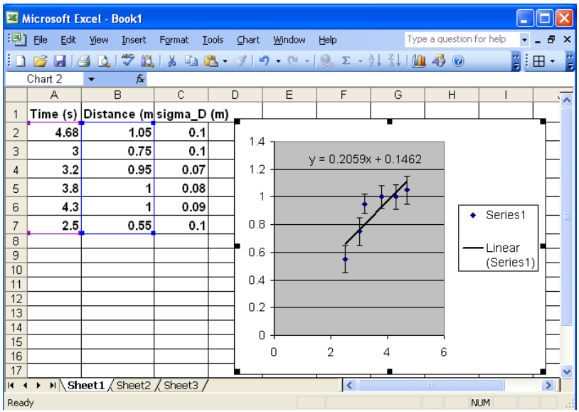
Figure 1: Adding an equation and trendline