
Conservation of Momentum
Purpose
-
•To investigate the behavior of objects colliding in elastic and inelastic collisions.
-
•To investigate momentum and energy conservation for a pair of colliding carts.
-
•To investigate the effect of the type of collision on the change in kinetic energy of a system of colliding carts.
Equipment
- Virtual Momentum Track
- VPL Grapher
- Pencil
Simulation and Tools
Open the Virtual Momentum Track simulation to do this lab. You will need to use the VPL Grapher to complete this lab.Explore the Apparatus
Open the Virtual Momentum Lab. A lot should look familiar after having worked with the Dynamics Track.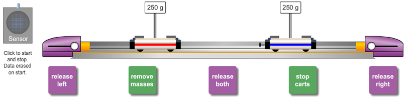
Figure 1: Carts, track, and motion sensor in the Virtual Momentum Lab simulation
-
•Turn on the "Motion Sensor" by clicking it.
-
•Release the left launcher.
-
•Once the carts collide, turn off the "Motion Sensor."
-
•You should see a graph similar to the one shown in Figure 2.
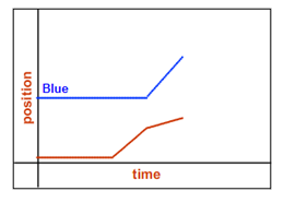
Figure 2
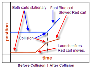
Figure 3
1
In the momentum apparatus, click Copy Data to Clipboard.
2
Open Grapher. Click in the "paste data" box and use Ctrl+V to paste it into the data table.
3
You should see three columns of data labeled "X," "Blue," and "Red." These hold the data for time, blue cart position, and red cart position, respectively. You should also see two graphs—one position-time graph for each cart. Use manual scaling to make sure that each graph starts at (0, 0) and has the same maximum x and t values. A range of 0.0 m to 2.0 m is good. Label the axes of the top graph "Blue Position (m)" and "Time (s)." Label the bottom graph similarly. Give each graph an appropriate name.
4
Turn on "Linear Fit." Determine the constant velocities of the carts prior to the collision by finding the four slopes of their (t, x) graphs. You should know how to use the "Linear Fit" tool from your kinematics labs or by studying the Lab Guide. You'll note that when you drag across a certain portion of the graph, a pink line of best fit is drawn for that range of points. The data in the "Linear Fit" data box also corresponds to that data range. Thus you can determine before-and-after-collision velocities for each cart. The longer the line segment you drag across, the better your results will be.
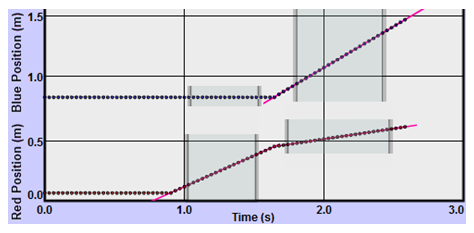
Figure 4
Theory
Momentum
In class and in your reading, you've seen the following development of the concepts of momentum, momentum conservation, and their connection to energy conservation. (Vectors are shown in bold type.) The momentum, p, of a body of mass, m, and velocity, v, is written asCase 1: A net external force acts on a body.
When a (net) force acts on a body, its velocity and hence its momentum will change according to equation 2. where FΔt is referred to as the impulse, J. Note that the impulse is a vector and is equal to the difference in two momentum vectors, pf and po. In words, equation 2 saysCase 2: An internal force acts between two bodies (or more than two, but that's out of our league).
As you know, forces come in equal and opposite pairs. So you know that in case 1 you were just focusing on one of the bodies involved. That's great for determining things like the effect of the force on a golf ball hit by a golf club. There are also many situations where it's useful to look at both bodies involved. If you want to slow down or change the course of an incoming asteroid, you need to know how big an object you need to throw at it, how fast you need to throw it, and in what direction. In these cases, the impulse on the system is zero since all forces are internal to the system. When there is a no net, external force, That is, there is no impulse, so there will be no change in momentum. Thus the momentum of the system is conserved.
So, if there is no net, external force on the system, the momentum of the system will remain unchanged even if the parts of the system exert forces on one another and the individual parts change their momentum.
Kinetic Energy
You've also become familiar with the kinetic energy, KE, of an object. The equation for kinetic energy involves the same terms, m and v. So, shouldn't the kinetic energy of the system always be conserved, too? That is, shouldn't it be the same before and after an interaction? No. There's a subtle difference between the equation mv for momentum and| 1 |
| 2 |
Procedure
Please print the worksheet for this lab. You will need this sheet to record your data.
I. Conservation of Momentum in a Collision
Note:
In most of this lab, you'll use your data to answer questions, even non-numerical questions.
In most of this lab, you'll use your data to answer questions, even non-numerical questions.
Δp1 = −Δp2.
say the same thing, but in two different ways. Let's explore both.
1
Load the blue cart with 500 g, giving it a total mass of 750 g. (Remove any mass that has been added to the red cart.)
2
Position the blue cart right between the release both and stop carts buttons.
3
Engage the red cart with its launcher. Cock the launch spring about halfway back.
4
Turn on the "Motion Sensor."
5
Release the left cart.
6
Somewhat before the blue cart hits the right bumper, turn off the "Motion Sensor." Your graph should look something like Figure 5.
There may be additional lines due to collisions with the plungers. Ignore them. Dragging the big white ball below the graph will adjust the time display scale.
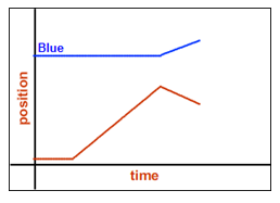
Figure 5
7
What is the sign of the red cart's initial momentum, mRvRo, its momentum just before the collision?
8
What is the sign of the red cart's final momentum, mRvRf, its momentum just after the collision?
9
What is the sign of the change in the red cart's momentum, Δ(mRvR) = mR(ΔvR)?
10
The blue cart's initial momentum, mBvBo, doesn't have a sign. What is its momentum before the collision?
11
What is the sign of the blue cart's final momentum, mBvBf, its momentum just after the collision?
12
What is the sign of the change in the blue cart's momentum, Δ(mBvB) = mB(ΔvB)?
13
Copy+Paste your data from the apparatus into Grapher as before. Using the "Linear Fit" tool, determine the carts' velocities before (Vo) and after (Vf) the collision. Record these in Table 1.
14
Using the known masses calculate and record the momentum of each cart before and after the collision (4 values).
15
Add the initial momenta of the carts to determine the initial momentum (p(sys)o) of the system. Similarly determine the final momentum (p(sys)f) of the system. Record these two values in Table 1.
16
Finally, calculate and record the change in momentum of the system (Δpsys) from (p(sys)f) – (p(sys)o).
17
Equation 6p1o + p2o = p1f + p2f. says that p(red)o + p(blue)o = p(red)f + p(blue)f. How did that work out? Quote your numbers.
18
Equation 7Δp1 = −Δp2.
says that p(red)f – p(red)o = –(p(blue)f – p(blue)o). How did that work out? Quote your numbers.
II. Elastic Collisions
With the "Spring Plunger," the carts seemed to bounce nicely off of each other. Could this have been an elastic collision, that is, one where the kinetic energy of the system was unchanged during the collision? Let's do the math and see.1
Table 2 works just like Table 1 and uses the same data. By filling in Table 2, you'll calculate the total KE of the system of two carts before (KE(sys)o) and after (KE(sys)f) the collision. You'll also calculate the change in kinetic energy of the system, ΔKEsystem, which is KE(sys)f – KE(sys)o. Note that in the equation for KE, only the speed is considered. That is, KE has no direction associated with it. This actually doesn't matter in your calculations since all the velocities are squared.
2
Does the kinetic energy of the system appear to be conserved in this collision? How do you know? Quote your numbers.
III. Totally Inelastic Collisions
In the previous section, we observed carts making elastic collisions. We found that both momentum and kinetic energy were conserved. Our carts can have another type of collision. The springy bumpers between them can be replaced by sticky "Velcro®" bumpers. In this case we would have a totally inelastic collision, one where the carts stick together after the collision and share a common speed.1
Let's start with the simplest case – a collision between carts of equal mass and equal but opposite velocities. Attach both carts to their launchers. Remove all extra masses. Fully cock both launchers (to provide equal initial speeds). Using the usual procedure, produce a graph of their head-on collision. You'll need to use the release both button.
-
aCopy and paste your data into Grapher. Add axis labels and an appropriate title to each graph. Manually adjust the y-axis scale on both graphs to range from 0.0 m to 2.0 m.
-
bTake a single Screenshot
 of the graph from Grapher and upload it as "Mom_III1.png".
-
cDraw the position-time graph produced by the apparatus in Graph III1.
-
dExplain how you know from the graph(s) that momentum was conserved, but kinetic energy was not. You should be able to tell just by looking at the graphs, but you can use Grapher to assist you.
Figure Graph III1: Head on Equal speed collision
2
Now try a similar collision, but this time with the blue cart initially sitting still at the center of the track.
-
aCopy and paste your data into Grapher. Again manually adjust the y-axis scale on both graphs to range from 0.0 m to 2.0 m. Add axis labels and an appropriate title to each graph.
-
bTake a single Screenshot of the pair of graphs from Grapher and upload it as "Mom_III2.png".
-
cDraw the position-time graph produced by the apparatus in Graph III2.
-
dThis one's not so obvious. You'll need some data and calculations to work with. Use Grapher to get the data you need. Use Table 3 to record your data and calculated values.
Figure Graph III2: Collision with stationary cart
3
Using your data, explain how you know that momentum was conserved, but kinetic energy was not conserved.
4
You should have found that the pair of carts moving as one with a mass of 2 × mcart had half the speed of the single cart with a mass of 1 × mcart. Why then is the kinetic energy less after the collision? That is, why doesn't one cart with a speed of v have the same kinetic energy as two carts each with a speed of | v |
| 2 |
5
For the situation in Graph III1, what fraction of the kinetic energy of the carts remains after the collision? That is, what is (KEfinal/KEinitial)? You don't have any numbers to work with, but you don't need any.
6
For the situation in Graph III2, what fraction of the kinetic energy of the carts remains after the collision? That is, compute (KEfinal/KEinitial). You'll need to use your numbers this time.