
Dynamics – Free Fall, Apparent Weight, and Friction (Honors)
Purpose
-
•To investigate the vector nature of forces.
-
•To practice the use of free-body diagrams (FBDs).
-
•To learn to apply Newton's Second Law to systems of masses.
-
•To develop a clear concept of the idea of apparent weight.
-
•To explore the effect of kinetic friction on motion.
Equipment
- Virtual Dynamics Track Simulation
- VPL Grapher
- Pencil
Simulation and Tools
Open the Virtual Dynamics Track simulation to do this lab. You will need to use the VPL Grapher to complete this lab.Explore the Apparatus
Open the Virtual Dynamics Track simulation. You'll see the low-friction track and cart at the top of the screen. At the bottom you'll see a roll of massless string, several masses, and a mass hanger. Roll your pointer over each of these to view the behavior of each. Note the values of the masses. Also note that the empty hanger's mass is 50 g. If you move your pointer over the cart, you'll see that its mass is 250 g.1
Drag the cart near the left end of the track.
2
Drag the spool of massless red string somewhere just to the right of the cart (Figure 1a). Release it by releasing your mouse button. A segment of string will attach to the cart and find its way over the pulley. A small loop (Figure 1b) will form at its lower end.
3
Drag the mass hanger until its curved handle is a bit above the loop (Figure 1c). Release your mouse button and the hanger will attach (Figure 1d). The cart will take off. It's alive! Drag the cart back and forth. Everything should work just as you'd expect.
Give it a toss or use Go to launch it with a known initial negative velocity.
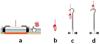
Figure 1
4
Check out the Brakes On/Off toggle button.
5
Try Reset All.
6
Reattach the string and hanger.
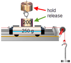
Figure 2
7
Toss the cart around and notice how it moves. Experiment with a variety of masses on both the cart and hanger. Investigate what determines the system's acceleration. You know how to add masses. You can remove them just by clicking. Try this. Turn on the brakes to hold the cart still and then add two masses to the cart and to each hanger. Click once on each of the three. The top mass will disappear in each case. Another three clicks will empty them all. Clicking on an empty hanger will remove it. The Reset All button will then remove the massless string.
8
Restore your system to its simplest configuration—empty cart, string, and empty hanger. Turn on the brake and move the cart near the left bumper.
Procedure
Please print the worksheet for this lab. You will need this sheet to record your data.
IA. Drawing Force Vectors
We've found that writing down what we know and want to know is essential to successful problem-solving. But with forces, there's the added directional information that's best described with a figure. Figure 2 is a nice representation of what our apparatus looks like, but it doesn't show us the forces. Drawing force vectors can make it easier to identify the forces acting on systems. They also guide us in deciding which forces go into the equation ΣF = ma.Free-body diagrams
Click to turn on Dynamic Vectors. You'll want to leave Dynamic Vectors on most of the time during this lab. Adjust the check boxes in the apparatus to match Figure 3.
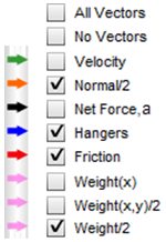
Figure 3: Vector Display Controls
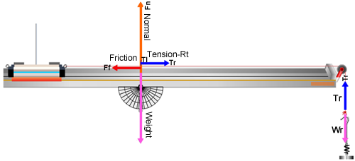
Figure 4: Dynamic Vectors
Cart Forces
In the vertical, you see the normal force, N, and the weight, W, which are equal and opposite. Thus there is no vertical acceleration by the cart, and there won't ever be with a level, indestructible track. (Fn and W are drawn half scale as Fn/2 and W/2 because they're so large and tend to go off the page.) Uncheck the "Normal" force and "Weight" vectors. In the horizontal, you see the tension in the (right) string, Tr and the friction force, Ff. They're also equal (while the cart is at rest) but opposite. Thus there is currently no acceleration in the horizontal because the brake is holding things at rest. Turn on the "Net Force" vector ( ) so that you can monitor ΣF and the acceleration once the cart starts moving. You'll just see the label "Fnet, a" but no vector arrow so far.
Hangar Forces
The forces on the mass hanger are the opposing forces Tr, and Wr. Wr is the weight of the right mass hanger. Tr is again the tension in the string. For a massless string, the tension is the same throughout. (For a non-massless string, the trailing end will have less tension than the leading end. We'll discuss that no further!) It's important that you understand that we use the term tension in two ways. In everyday use we think of the tension as the tautness of a string. That tautness is caused by forces pulling on each end. The reaction force by the strings' ends on the cart and hanger are also referred to as the tension. So we say that the tension force provided by the string acts equally (for our massless string) on both the cart and the hanger. So the pair of T's will always represent equal magnitude forces acting on the objects the string is attached to. Make sure that you see how that's represented in Figure 4.The System
Newton's Second Law, ΣF = ma, describes the effect of a net force on an object or group of objects, referred to as the system, that move with some acceleration, a, due to the net, external force, ΣF, acting on the system. The mass, m, is the total mass of the system. For a system of more than one object Newton's Second Law works for the whole group or any part of the group.-
aIn Figure 5, we might consider the cart and hanger as a system and then consider the net, external force on that system, and the mass of the system.
-
bWe might also say, "let's consider just the cart as the system." We'd then look at the forces on the cart, the cart's mass, etc.
-
cIn this lab, we'll think of the cart and hangers as "the system" unless stated otherwise.
The Net Force
In Figure 4, the cart-hanger system remained at rest because of the brake which exerts a friction force, Ff, which changes to match any amount of weight that can be added to the hanger. When you release the brake the vectors should change to look like Figure 5. Try it at few times. There is now a net force, so there will be an acceleration. Try turning the brake on and off and notice how the forces change. You can also just hold and release the cart with the mouse. You're sort of acting like a brake but no vector will be shown to represent this.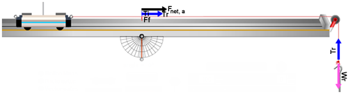
Figure 5: The Net Force
IB. Accelerated System of a Cart on a Level Track with Mass Hanger and No Friction
Let's see how we can use FBD's to help us think about a simple system and then build some equations to describe it mathematically. Set up the system shown in Figure 6. You need a level track with an empty hanger on the right and an extra 200 g on the 250-g cart.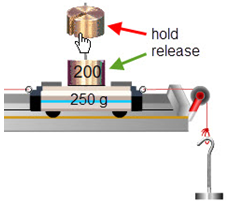
Figure 6: Adding Cart Masses
1
Although the cart and hanger are moving in different directions, they're otherwise moving identically. For example, when the hanger is moving at, say, 2 m/s, the string ensures that the cart is also moving at 2 m/s.
2
This also includes direction, if you don't mind a minor 90° bend in the middle. Motion left and right by the cart is the same as motion up and down by the hanger. The pulley is just redirecting it. We'll work with the bendy direction and say that the positive direction is as shown in Figure 7. For the cart, the +x-direction is to the right. For the hanger, it's downward.
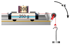
Figure 7: the "x-direction"
3
We don't know the net force on either object but if we look at the cart, string, and hanger as one system, there is only one unbalanced, external force acting on the system—the weight of the hanger. (The cart's weight and normal force cancel.) So our system behaves the same as the one shown in Figure 8 where the masses of the cart and hanger make up the total mass and the weight of the hanger is the net force.
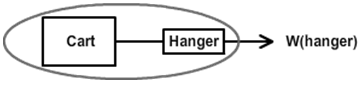
Figure 8: The System Mass (Note the cool optical illusion. The squares don't look quite square.)
OK, let's use the cart and hanger as our system. Think about these three questions.
-
amsystem = ?
-
bΣFon system = ?
-
casystem = ?
-
aClearly, both the cart and hanger are accelerating. Somsystem = 450 g + 50 g = 500 g = 0.500 kg.(Note the mks units.)
-
bThere are three forces present: Tr, Tr, and Wr. But both Tr's are internal to the system. The only external force is Wr.Wr = mhangerg = 0.050 kg × 9.80 N/kg = 0.49 N.
-
ca =
=Σ F (mcart + mhanger)
= 0.98 m/s20.49 N 0.500 kg
Confirm these results experimentally.
Using your virtual apparatus, confirm your results. If you recall, in the acceleration lab you found the acceleration of a cart from the slope of a velocity-time graph. That would be a good method to use here.4
With the brake on, turn on the sensor. Then release the brake. Turn off the sensor when the cart reaches the bumper.
5
Copy Data to Clipboard and use Ctrl+V to paste it into Grapher.
6
Turn on Graph #2 to display the v-t graph. (Turn on Graph #3 just to shrink Graphs #1 and #2.)
7
Sketch the graphs you obtained from Grapher below.
8
Take screenshots of your x-t and v-t graphs. Save them as "Dyn_IB1a.png" and "Dyn_IB1b.png" and upload them. You can sketch them or attach printouts in the space provided.
Figure 9: Graph IB
9
Record the acceleration, the slope from the v-t graph.
10
Compare this with the theoretical (calculated value) above in 3c by calculating the percentage error.
11
Show your calculations for percentage error. Use the calculated value as the theoretical value.
Summary
The hanger's weight, Wr, is gravity's pull downward on the hanger, so it's an external force. That is, it's a force exerted on the system from outside. The two tension forces, Tr, are internal to our cart-string-hanger system, so they don't affect its motion. The system does include the string. The pulley changes the direction of the tension force but doesn't affect its magnitude. The net external force, Fnet is equal to Wr. Observe the moving cart and note that the lengths of their vectors are equal. Just to make sure you understand, the net force is not a particular force acting on our system. It's the sum of all the external forces. Also, we often leave off the term "external" and just say net force.IC. Accelerated System of a Cart on a Level Track with Two Mass Hangers and No Friction
How about adding a mass hanger on the left side?1
Set up your own arrangement and repeat the procedures in Part IB. Add masses to each hanger, choosing your hanger masses so that there will be a non-zero acceleration.
2
Provide a well-organized display showing
-
aall your data from the apparatus. This would just be all your masses.
-
ball your calculated values. This would include your total mass, all external forces affecting the acceleration, the net force on the system, calculated acceleration from ΣF = ma, experimental acceleration from the slope of your v-t graph, and the percentage error between the calculated (theoretical), and experimental values for your acceleration.Be careful with units!
-
call calculations involved in item 2b.
3
Take screenshots of your x-t and v-t graphs and upload them as "Dyn_IC1a.png" and "Dyn_IC1b.png". You can sketch them or attach printouts in the space provided.
Figure 10: Graph IC
IIA. Free Fall Acceleration
We've found that all bodies in free fall have the same downward acceleration, g. Let's use our apparatus to find the value of g for a falling mass hanger. We need a system of one object—the mass hanger. Hmm. You can't have a mass hanger without a string to attach it to. And all position measurements are associated with the cart, not the hanger. So we need a cart, but not its mass. We need a sort of vacant, empty, soulless, massless cart. What we need is a Zombie CART! Or as Dr. Seuss would call it, little cart Z.1
Set up the Dynamics Track with an empty cart and hanger. Drag the cart near the left bumper and let it go. That looks OK, but as noted, the hanger is not really free falling. It's dragging the cart behind it.
2
Put on the brake and move the cart near the left end of the track. Now click on the Z-cart icon. The cart will become translucent indicating that it has become massless. Zoom! Clicking the Z-cart icon again will restore its mass. Repeat in and out of Z-mode to convince yourself that the whole system seems to move with a greater acceleration, possibly equal to g, when the cart's mass is eliminated. That's because the system here is really just the mass hanger. So the Z-car is doing just what we want it to do. It's collecting sensor data without contributing any mass.
3
Try this. Turn on the motion sensor and record the motion in normal mode (hanger + normal cart) in one color. Then, select another line color and try a Z-mode run. Do the graphs show different accelerations? They should.
4
You may have noticed that the brake doesn't work in Z-mode. Check it out. Why doesn't it work in Z-mode?
5
Since we can eliminate the mass of the cart with Z-mode, we can now look at the motion of the freely falling hanger. Find its acceleration as follows.
-
aSet "Recoil" to zero to eliminate bouncing.
-
bUse normal mode (not Z-mode) with an empty cart and hanger. Move the cart near the left end of the track with the brake on.
-
cTurn the motion sensor on.
-
dClick on the Z-cart icon. The cart should quickly accelerate to the right end of the track.
-
eTurn the motion sensor off.
vo ≈ 0.
So
We can get Δt and Δx from the Dynamics Track data table. Look at the position values. They're all the same until you turned off the brake.

Figure: Sample Data
6
Find the last data pair before the cart starts moving. Ex. x = 0.098, 0.098, ..., 0.098, 0.108 ← the last 0.098. This will be our initial value, when vo ≈ 0. The cart's motion actually started between this instant and the one after it, but we'll get a fairly accurate number if we ignore this error.
-
aRecord this first data pair as t1, and x1 in Table 4 in WebAssign.
-
bScroll through the data to find a point somewhat before the cart hit the right bumper. That is before the position stops changing. Record the data for this point as t2, and x2 in Table 4 in WebAssign.
-
cCalculate and record Δx, and Δt in Table 4 in WebAssign.
-
dCalculate and record the acceleration using equation 2 in Table 4 in WebAssign.
7
Record the following: system mass (mass hanger), m; net force, ΣF = mg; theoretical a = F/m.
8
Show calculations using equation 2Δx ≈
a Δt2.
for the acceleration with just the mass hanger.
| 1 |
| 2 |
9
Show calculations for percentage error. Use the F/m value for acceleration as your theoretical value.
Your result should be somewhat different than the theoretical value since the timer was already counting when we started the cart so the time when the cart actually started was most likely in between two time readings.
IIB. Free Fall – The Effect of the Weight of the Falling Object on Its Acceleration
Throughout most of recorded history, it was believed that the heavier a body is, the faster it will fall. (Those of that opinion also didn't quibble over the definition of the terms "fast" and "slow." Did it correspond to velocity or acceleration?) At first glance, F = ma would seem to support their theory since the acceleration is directly proportional to F. Thus, a heavier body would seem accelerate faster than a lighter body. Let's test this old theory. In Part IIA, you observed the fall of the empty mass hanger. Let's make it heavier to see if it goes "faster" (greater acceleration).1
Double the weight of the hanger by adding a 50-g mass to it. (You'll have to turn off Z-mode temporarily to allow you to put mass on the hanger.)
2
Change graph colors so that you can see the new graph along with the previous one. Take your data and record it as before, but in Table 5 in WebAssign. Calculate and record the free fall acceleration of the 100-g mass.
3
Compare Tables 4 and 5 in WebAssign. Doubling the force did not seem to double the acceleration. If a ∝ F, we must be missing something.
-
aThe _____ of a body is directly proportional to the net force acting on it.
-
bSo if you double the force on it, its acceleration should _____.
-
cWhen you doubled the mass in this case, the acceleration _____.
-
dThis is because doubling the weight also doubled the _____.
IIIA. The Roles of Newton's Second and Third Laws in Identifying the Forces Affecting Motion
Anyone who's ridden in an elevator is familiar with the light or heavy feeling during the elevator's upward or downward acceleration. To understand the source of this feeling and why it makes us feel like our weight has changed, it's important to be clear about the forces involved. In Figure 11, we have the two opposing forces acting on our mass hanger. Are they an action-reaction pair? No! And not just because they aren't necessasarily equal. Since each force must be associated with an equal and opposite reaction force, there must be some other forces involved.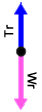
Figure 11: FBD
Newton's Second Law:
ΣF = ma, where ΣF is the sum of the forces on a body (or system) with mass m. These forces may or may not be equal. They all act on one body.
ΣF = ma, where ΣF is the sum of the forces on a body (or system) with mass m. These forces may or may not be equal. They all act on one body.
Newton's Third Law:
Body 1 exerts a force on body 2. Body 2 exerts an equal but opposite force on body 1. The third law helps us identify all the forces involved in an interaction between bodies.
Body 1 exerts a force on body 2. Body 2 exerts an equal but opposite force on body 1. The third law helps us identify all the forces involved in an interaction between bodies.
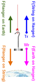
Figure 12: All Forces on Hanger
( A-R pair #1 )
F (hanger on Earth) = –F (Earth on hanger), Wr
( A-R pair #2 )
F (hanger on string) = –F (string on hanger), Tr
-
aDecide which object you're interested in. (the hanger)
-
bUse just the forces acting on it.
IIIB. Apparent Weight
Now suppose that instead of the mass hanger, you were clinging to the end of string. You are the dot in the figure. Gravity pulls you downward with a force, Wr. The string pulls up with a force, Tr.
That force Tr is what we call your apparent weight.
Wr is your actual weight, mg.
1
Set up the system shown in Figure 13.
-
aYou'll want a string and empty hanger on each side.
-
bYou'll want Z-mode for this activity. Also recoil = 0.
-
cTurn on Dynamics Vector. Check (turn on) "Hangers" and "Velocity."
-
dThese vectors get in the way of the left hanger. The column of arrows that identify the vector colors is also a toggle to show/hide the check boxes. You might want to hide them.
-
eAdd 50 grams to each hanger You're on the right. Your mass (mr) is 100 g!
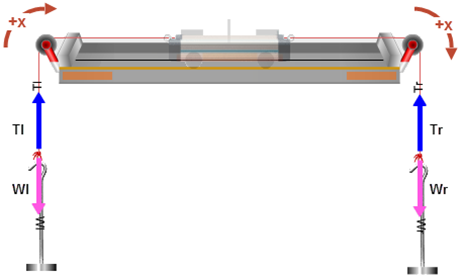
Figure 13: Apparent Weight
2
Let's look at the initial situation—hanging from the rope at rest. That is, vo = 0 and constant.
- a = 0, so Tr = Wr.
- Note the length of these vectors on the right side. They're equal since a = 0.
3
Now give the cart a good shove in either direction. Or use "Vo" and Go →.
4
How does your apparent weight (Tr) at rest compare to Tr when moving at a constant velocity?
From this you should conclude that your apparent weight, Tr should be your normal weight. This means that if you were hanging from the string, you wouldn't feel any more stretched out moving at a constant speed than when at rest. Likewise if you were standing on the scale, you wouldn't feel any more squished down by gravity than usual.
5
Now try an upward acceleration. Add 100 grams to the left hanger. You should now have a total of 100 g on the right and 200 g on the left. Drag the cart to near the right end of the track. Ignore the situation when Tr = Wr when the cart is being held. You want to notice what happens just when you release the carts.
6
Answer the following questions.
-
aWhen you release the cart, what happens to your apparent weight, Tr? (increases, decreases, or remains the same)
-
bWhen you release the cart, what happens to your actual weight, Wr? (same choices)
-
cWhat would it be like, relative to when you were riding at a constant speed, if you were hanging from the string or standing on the hanger? (stretched or compressed)
7
Now try a downward acceleration. Adjust the masses so that the right side is still 100 g and the left side is an empty 50-g hanger. Drag the cart to near the left end of the track.
-
aWhen you release the cart, what happens to your apparent weight, Tr? (increases, decreases, or remains the same)
-
bWhen you release the cart, what happens to your actual weight, Wr? (same choices)
-
cWhat would it be like, relative to when you were riding at a constant speed, if you were hanging from the string or standing on the hanger? (less stretched or less compressed)
8
When you accelerate upward your apparent weight _____.
9
When you accelerate downward your apparent weight _____.
10
When you are at rest or moving at a constant speed your apparent weight is _____.
IV. Kinetic Friction
And finally, let's have a quick look at kinetic friction. For this study we'll just be working with the normal cart. The only force affecting its motion will be kinetic friction. So click Reset All to remove all the masses and hangers. So far the only friction force we've encountered is the one supplied by the cart brake. It's much too strong a force for our purposes. Instead, we'll use a friction pad similar to the brake. But this one is adjustable. In Figure 14, you see a snapshot of the cart traveling to the right at velocity vo. A friction force, the net force, acts to the left, thus slowing the cart down.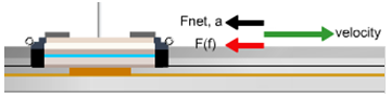
Figure 14: Friction Pad
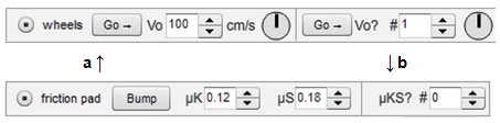
Figure 15: 15a (with wheels), 15b (with fraction pad)
1
Click the "friction pad" radio button to turn on the friction controls. Set the friction controls as shown in Figure 15b.
2
Turn on the ruler. Move it above the Dynamic Vectors display.
3
Move the cart to x = 10.0 cm. (This is the position of the cart mast.)
4
Turn on the Dynamic Vectors tool:
. Check (turn on) "Velocity," "Net Force," and "Friction."
5
Click "wheels" and set "Vo" to 200 cm/s. Then switch back to "friction pad."
6
Click Go. The cart should launch to the right and slow to a stop before reaching the right bumper. If not, retry the preceding instructions.
7
Repeat the preceding step as needed to answer the following.
8
Clearly the cart slows down. What about the friction vector, Ff, tells you why it slows down.
9
What about the velocity vector tells you that it does slow down.
ΣF = ma
Ff = ma
Ff = − μkFN = −μkmg
−μkmg = ma
- vo = 2.00 m/s.
- vf = 0.00 m/s.
- Δx can be found with the ruler.
- a can be found from a single kinematics equation. You figure that part out.
10
Got it? Take the data you need and record it. If your value for μk is not close to 0.12, then you've done something wrong with your technique or your calculations. You should get a negative value for the acceleration. (Use g = 9.80 m/s2.)
11
Let's try an unknown friction coefficient. Change the "μKS?" value to 2 using the numeric stepper. You'll quickly find that your 2.00 m/s is not a good choice this time. You can change it to whatever you like. But letting the cart go most of the way along the track will give better results than a short run. Note also that the new μks should be much smaller than the previous value. Record your data and calculations. (Use g = 9.80 m/s2.)