Lab 10 - The Ideal Gas Law

Introduction

The volume of a gas depends on the pressure as well as the temperature of the gas. Therefore, a relation between these quantities and the mass of a gas gives valuable information about the physical nature of the system. Such a relationship is referred to as the equation of state. One of the most fundamental laws used in thermal physics and chemistry is the Ideal Gas Law that deals with the relationship between pressure, volume, and temperature of a gas.

Discussion of Principles

Boyle's Law

Boyle's Law gives the relation between the pressure and volume of a given amount of gas at constant temperature. It states that the volume is inversely proportional to the pressure of the gas.

( 1 )

V ∝

where V is the volume of the gas and P is the pressure. This can also be written as

( 2 )

PV = constant.

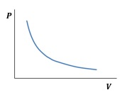
The plot of pressure versus volume is shown in Fig. 1 below.

Figure 1: Pressure versus volume plot

Charles's Law

Charles's Law states that the volume is directly proportional to the temperature T of a given amount of gas maintained at constant pressure.

( 3 )

V ∝ T

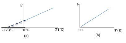
Figure 2a shows the plot of volume versus temperature in Celsius. Note that the graph is a straight line that when extrapolated back, intersects the horizontal axis at –273°C. At this temperature the volume of the gas goes to zero. This temperature is defined as the absolute zero temperature or 0 kelvin (0 K). The same graph is plotted using the Kelvin scale or absolute scale in Fig. 2b. Now the graph goes through the origin.

Figure 2: Plot of volume versus temperature

Gay-Lussac's Law

At constant volume, for a given amount of gas, the pressure is directly proportional to the temperature. This relationship is known as Gay-Lussac's Law and can be written as

( 4 )

P ∝ T

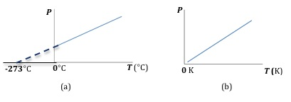
A plot of pressure versus temperature will be very similar to that of volume versus temperature. Again, note that in Fig. 3a, the straight line graph intersects the temperature axis at –273°C, and in Fig. 3b it passes through the origin.

Figure 3: Plot of pressure versus temperature

The Ideal Gas Law

The three gas laws discussed above can be combined to give a more general relation between the volume, pressure, and temperature of a gas.

( 5 )

PV ∝ T

Equation (5) describes the behavior of one variable when the other two variables are changed. If the temperature is kept constant, then this reduces to Boyle's Law. If the pressure or volume is kept constant, Eq. (5) reduces to Charles's Law or Gay-Lussac's Law respectively. The more general form of the gas law includes the amount of gas present and is expressed as

( 6 )

PV = nRT

where R = 8.314 J/(mol·K) is the universal gas constant and n is the number of moles of the gas. n can be calculated using the definition

( 7 )

n(mol)=

mass (grams)

molecular mass (g/mol)

Note: If the pressure is in pascals, Pa, the volume is in m³, n is in mol, temperature is in Kelvin, and R is 8.314472 J/(mol·K).

Adiabatic Compression

Adiabatic compression happens when a gas is compressed so quickly that all the work put into the compression goes into heating the gas, i.e. no heat escapes to the outside environment during compression. For adiabatic compression the pressure and volume are related by:

( 8 )

P_iV_i^γ = P_fV_f^γ

where

is the ratio of specific heats. For air

γ ≈ 1.40.

Objective

The objective of this experiment is to measure the volume and pressure of a given amount of gas for constant as well as varying temperatures and study the relation between pressure, volume, and temperature of a gas.

Equipment

DataStudio software
Pasco pressure sensor
Science Workshop 750 interface
Computer

Procedure

In the first part of the experiment you will maintain a constant temperature and measure the pressure for two different volumes. From this you will determine the correction to be applied to account for the tubing portion of the apparatus. In the second part, you will measure the pressure and temperature for two different volumes and verify the ideal gas law. In part three you will determine the number of moles of gas in your apparatus from a plot of volume versus pressure. Finally, in the last part you will examine the behavior of the gas when it is subjected to adiabatic expansion.

Description of apparatus

The apparatus is comprised of a plastic syringe with a plunger, a pressure sensor and a temperature sensor. See Fig. 4 below. The end of the syringe is connected via plastic tubing to a pressure couple, the other end of which is connected to the pressure sensor.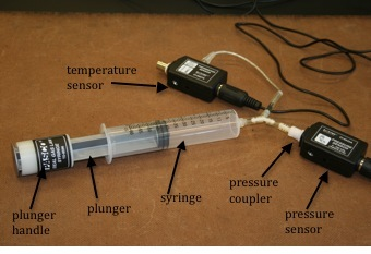

Figure 4: Photo showing the components of the apparatus

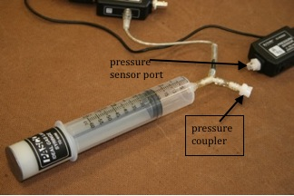
The syringe has graduations in cubic centimeters (cc) that allows for easy reading of the volume of gas in the part of the syringe below the plunger. To open the syringe to the atmosphere, you will have to disconnect the tubing from the pressure sensor. To do this, turn the connector counterclockwise and gently remove the coupler from the sensor. To reverse the operation, align the coupler with the pressure sensor port, push the coupler in and turn it clockwise until it clicks into place. Figure 5 shows the pressure sensor disconnected from the syringe tubing.

Figure 5: Syringe tubing is disconnected from the pressure sensor

Connect the pressure sensor unit to analog channel A of the Science Workshop Interface.

Open the appropriate DataStudio file associated with this lab. Figure 6 shows the opening screen in DataStudio.

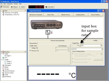
Figure 6: Opening screen for DataStudio software

Please read through all the steps in each part before you attempt that part.

Procedure A: Constant Temperature

In DataStudio, set the sampling rate to 20 Hz. See Fig. 6.

Disconnect the white plastic pressure coupler from the pressure sensor.

Press the plunger of the syringe all the way in as far as it will go. See Fig. 7 below.

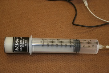
Figure 7: Plunger is pushed all the way in

Record this minimum volume as your final volume in Data Table 1. It should be close to 20 cc.

Move the plunger handle back to set the volume at 40 cc as shown in Fig. 8. Record this on the worksheet as the initial volume of gas.

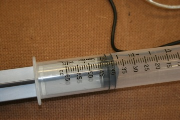
Figure 8: Plunger set at 40 cc

Now re-connect the coupler to the sensor.

Before you start collecting data, you might have to reposition the two graph windows, one below the other, to enable you to monitor them both simultaneously, as you collect data.

Click Start to record data and quickly compress the plunger all the way in and keep it compressed. The plunger handle should be all the way down and flush against the mechanical stop.

Monitor the graphs of pressure and temperature on the computer screen, and continue to hold the plunger in until the values stay constant. This should take about 10 seconds.

Once the temperature and pressure have equalized, release the plunger. Again, monitor the graphs and wait until the values remain constant.

Click Stop to stop the data collection.

Figure 9 shows the general shapes of the two graphs.

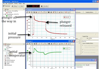
Figure 9: Screenshot showing the two graphs

The initial pressure of the gas is the pressure before you compressed the air when the volume was at 40 cc and the gas was at room temperature. Read this initial pressure from the pressure versus time graph and record this in Data Table 1.

The final pressure of the gas is the pressure just before you released the plunger. Read this final pressure from the pressure versus time graph and record this in Data Table 1.

The final volume is the volume that the plunger stopped at in step 6, and the temperature should be at room temperature at this point in your data collection. Record these values in Data Table 1.

The amount of air and the temperature in the syringe are the same at the initial point and the final point. On the worksheet write down the ideal gas law in terms of

P_i, V_i, P_f, and V_f.

The experimental error in this syringe is due to the unknown volume

V₀

of the tubing. Rewrite the equation from step 17 to include this additional volume.

Solve this equation for

V₀.

Your answer should be in terms of

P_i, V_i, P_f, and V_f.

Use the values for

P_i, V_i, P_f, and V_f

from Data Table 1 to calculate

V₀

and record this on the worksheet.

Checkpoint 1:
Ask your TA to check your table values and calculations.

Procedure B: Varying Temperature

Highlight an area on the temperature graph at the beginning of the run before you compressed the air.

Record these initial values of the pressure and temperature in Data Table 2.

Record the initial volume

V_i.

Be sure to include the value of

V₀

that you calculated in step 20.

Consider the portion of the temperature versus time graph when you released the plunger.

Highlight the area on the graph where the temperature peaks.

Record the peak temperature

T_f

and the corresponding pressure

P_f

at the time the temperature peaked in Data Table 2.

Record the volume

V_f

including

V₀

of the fully compressed plunger in Data Table 2.

In this case only the amount of air is constant in the syringe.

What does the ideal gas law algebraically reduce to in terms of

P_i, V_i, P_f, and V_f?

Write this down on the worksheet.

Calculate the quantity

P_iV_i

T_i

using the values from Data Table 2.

Calculate the quantity

P_fV_f

T_f

using the values from Data Table 2.

Find the percent difference between the two values found in steps 26 and 27 and record this on the worksheet.

Checkpoint 2:
Ask your TA to check your table values and calculations.

Procedure C: Determining the Amount of Gas

Add a digits display of temperature in DataStudio.

The digits window might be behind the graphs. Double-click Digits on the left side of the DataStudio window to activate the Digits window. See Fig. 10.

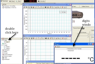
Figure 10: Adding the digits window

Disconnect the white plastic coupler from the pressure sensor.

Set the plunger at 45 cc and re-connect the coupler to the sensor.

You will decrease the volume in steps of 5 cc and each time you will wait for the temperature to come down to room temperature. Do not release the plunger between each step.

Start recording data.

Compress the plunger to 40 cc and hold it at this position. Watch the temperature on the digits display and wait until it drops down close to room temperature.

Note the final (equilibrium) temperature. Each time you compress the air in this sequence wait until the temperature returns back close to this value.

Compress the plunger further to 35 cc and hold it in this position until the temperature drops to the value you noted in step 32. Do not release the plunger.

Repeat step 33 by pushing the plunger to 30 cc, 25 cc, and finally to 20 cc.

Click Stop to stop recording data.

Pressure versus time and temperature versus time graphs for part of this process is shown in Fig. 11.

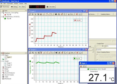
Figure 11: Pressure and temperature graphs for Procedure C

Compare your temperature and pressure graphs to determine when the plunger was at 40 cc. The values of temperature and pressure will be your equilibrium values. Record these in Data Table 3.

Repeat step 36 for all the other volumes including

V₀

found in Procedure A. Pick a temperature as close to the equilibrium temperature as possible and record its corresponding pressure. Record these values in Data Table 3.

Calculate 1/P for each of the volumes and record these values in Data Table 3.

Use Excel to graph volume versus 1/P. See Appendix G.

Use the Linest function to determine the slope of the graph and record this on the worksheet. See Appendix J.

From the slope determine, paying particular attention to the units, the number of moles in your syringe.

Checkpoint 3:
Ask your TA to check your table values, graph, and calculations.

Procedure D: Adiabatic Compression

Set the sample rate at 50 Hz.

Disconnect the white plastic coupler from the pressure sensor.

Set the plunger to 60 cc and then re-connect the coupler to the sensor.

Click Start and as quickly as possible compress the plunger from 60 cc down to 20 cc. Do this in one quick motion until the plunger handle is all the way in.

Click Stop to stop recording data.

Your graphs should resemble the ones shown in Fig.12 below.

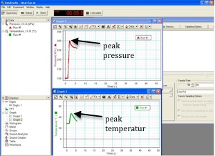
Figure 12: Graphs for adiabatic compression

Use your pressure and temperature graphs to find the initial values of the pressure and temperature before you compressed the syringe. Record these values in Data Table 4.

Record the initial volume including

V₀

from Procedure A in Data Table 4.

Use the graph to find the peak temperature and the peak pressure. Record these in Data Table 4.

Use your values for

P_i, V_i, and V_f

to calculate the theoretical peak pressure

P_f.

Compare the theoretical peak pressure to the peak pressure you recorded in Data Table 4 by finding the percent difference between these two values.

Checkpoint 4:
Ask your TA to check your table values and calculations.