
Module 1 – Motion
Introduction
One important topic of this module is motion. In this experiment, you will be studying two special types of motion.-
1Motion with constant velocity
-
2Motion with constant acceleration
NOTE:
Before proceeding to the rest of the experiment, make certain that you have read Section 1.4 in your text.
Before proceeding to the rest of the experiment, make certain that you have read Section 1.4 in your text.
Motion with Constant Velocity
Motion with constant velocity is also called uniform motion. Let's take a look at some of the most important aspects of uniform motion which result from constant velocity.-
1Both the speed and direction of motion do not change.
-
2The acceleration is zero.
-
3The distance moved each second is the same.
-
4The equation of motion which describes uniform motion isd = vt, where v is a constant value, such as 8 m/s.
y = mx.
If you plot the distance an object moves along the vertical axis and the time it takes the object to move that distance along the horizontal axis, then the d vs. t graph of uniform motion will be a straight line with a slope equal to the velocity of the object. Take another look at the two equations.
Position vs. Time Graph of Uniform Motion
Look at the figure below. It illustrates how the shape of the d vs. t graph changes as the speed changes for a body with constant velocity.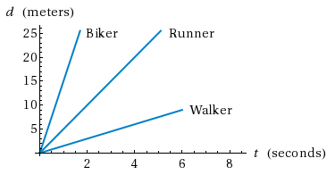
Figure 1
Calculating Velocity (Uniform Motion)
Let's take a look at another illustration. This illustration shows you how to calculate the velocity of an object by finding the value of the slope of the position vs. time graph. Notice that the distance traveled each second is about 8 m. At the end of 1 second, the distance traveled is 8 m; at the end of 2 seconds, the distance traveled is 16 m, and so on. This is characteristic of uniform motion. Each second the distance traveled is the same.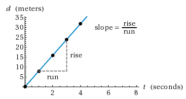
Figure 2
v = d/t
or v = Δd/Δt.
The change in distance is just the rise of the graph between two points and the change in the time is the run of the graph between two points.
Linear Motion with Constant Acceleration
The second type of motion we will study is uniformly accelerated motion, or motion with constant acceleration in a straight line. The key aspects of this type of motion are:-
1The speed changes but direction does not change. The acceleration is not zero but it does not change.
-
2The acceleration can be negative or positive.
-
3The distance moved each second changes.
-
4The change in velocity is the same from second to second.
-
5The equation which describes velocity at any time isv = at,where a is a constant value, such as 3 m/s2.
Velocity vs. Time Graph of Uniformly Accelerated Motion
The figure below shows the linear relationship between velocity and time when acceleration does not change. If we re-write the equation for velocity, we get:a = v/t
or a = Δv/Δt.
In other words, the slope of the velocity vs. time graph corresponds to the acceleration. This is true for all motions, not just uniformly accelerated motions.
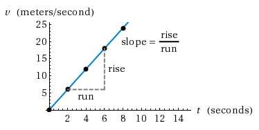
Figure 3
Position vs. Time (Uniform Acceleration)
Some students wonder what the position vs. time graph looks like for uniformly accelerated motion in a straight line. After all, we discussed the position vs. time graph for uniform motion and some students wonder why we didn't discuss that graph for linear motion with constant acceleration. Let's take a look at the equation of motion which is relevant here. It turns out that the equation isd = 1/2at2
and the graph looks like this:
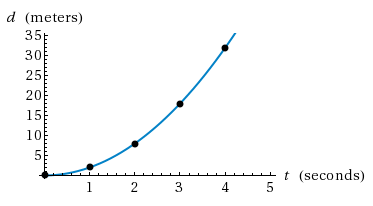
Figure 4
y = Cx2
are equations of parabolas. You may describe this graph as an increasing curve, if you wish, but the graph is also known as having a parabolic shape.
The slope of this graph at any point will be the velocity of the object at that point. Notice how the slope of the curve is always increasing. That is because the velocity is increasing since the object is undergoing acceleration.
Procedure
This experiment consists of three parts.1
Open the experiment instructions and worksheet.
-
•Motion Experiment Instructions (HTML or PDF)
-
•Motion Experiment Worksheet
2
After you have thoroughly read the instructions and worksheet, open the experiment simulation in which you will conduct the experiment and collect your data.
3
Record your data in the worksheet. (You will need it for the lab report assignment in WebAssign.)