Finding Normal Distribution Probabilities
To calculate probabilities for any normal distribution, standardize the appropriate interval endpoints and then use technology or the table of curve areas. More specifically, if is a variable whose behavior is described by a normal distribution with mean and standard deviation then
where is a variable whose distribution is standard normal and
Using the Table of Standard Normal Curve Areas
For any number between and 3.89 and rounded to two decimal places, the appendix table gives
where the letter is used to represent a random variable whose distribution is the standard normal distribution.
To find this probability using the table, locate the following:
- The row labeled with the sign of and the digit to either side of the decimal point (for example, or 0.5).
- The column identified with the second digit to the right of the decimal point in (for example, 0.06 if
The number at the intersection of this row and column is the probability,
Areas under the Normal Curve
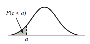
The probability that is less than is shown below.

A curve starts just above the horizontal axis, goes up and right, reaches a peak, goes down and right, and ends just above the horizontal axis. A point on the horizontal axis to the left of the peak is labeled a. The area under the curve and to the left of a is shaded and labeled P(z < a).
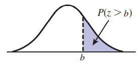
The probability that is greater than is shown below.

A curve starts just above the horizontal axis, goes up and right, reaches a peak, goes down and right, and ends just above the horizontal axis. A point on the horizontal axis to the right of the peak is labeled b. The area under the curve and to the right of b is shaded and labeled P(z > b).
Refer to the figure below for a visual explanation of the area under the normal curve between and

Three identical curves above three different horizontal axes are shown. All three curves start just above the horizontal axis, go up and right, reach a peak, go down and right, and end just above the horizontal axis.
- For the first curve, two points on the horizontal axis labeled a and b are to the left and right of the peak, respectively. The area under the curve and between these two points is shaded and labeled P(a < z < b).
- For the second curve, the same point b from the first curve is labeled on the horizontal axis. The area under the curve and to the left of b is shaded and labeled P(z < b).
- For the third curve, the same point a from the first curve is labeled on the horizontal axis. The area under the curve and to the left of a is shaded and labeled P(z < a).
- The three curves are displayed in a row: first, second, and then third. An equal sign is between the first and second curves and a minus sign is between the second and third curves.
Using SALT for Normal Distribution Probabilities
Click "Use SALT" to access SALT, and navigate to the Distribution Calculators tab.

A screenshot of the menu bar at the top of the SALT program is shown. The tab labeled "Distribution Calculators" is selected.
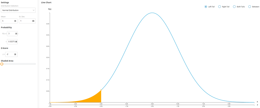
Based on the desired probability, determine the region of the area under the curve. For example, to find select Left Tail. Enter the given mean and standard deviation into the Mean and St. Dev. fields, respectively. Then enter the given value of The corresponding probability will be displayed in the probability section.

A screenshot of the Distribution Calculators page is given, where a menu labeled "Settings" is shown on the left. In the Settings menu, a drop-down list labeled "Distribution Selection" has the option "Normal Distribution" selected, and two text entry boxes labeled "Mean" and "St. Dev." have the numbers 5 and 1 entered into them, respectively. Below the Settings menu, another menu labeled "Probability" shows text reading P(x ≤ 3) = 0.02275 where the numbers 3 and 0.02275 in this text are being entered using two text entry boxes. Below the Probability menu, another menu labeled "Z-Score" shows text reading "z = −2" where the number −2 in this text is being entered using a text entry box. Below the Z-Score menu is a slider labeled "Shaded Area." To the right of the Settings menu, there is a set of radio buttons labeled "Left Tail," "Right Tail," "Both Tails," and "Between." The "Left Tail" button is selected. Below the radio buttons is a graph, which has a horizontal axis labeled x with values from 1 to 9 and a vertical axis labeled f(x) with values from 0 to 0.4. A second horizontal axis labeled z lies below the first and has values from −4 to 4. A curve starts just above the horizontal axis, goes up and right, reaches a peak above 5 on the x axis and 0 on the z axis, goes down and right, and ends just above the horizontal axis. The area under the curve to the left of 3 on the x axis (or −2 on the z-axis) is shaded.