Newton's Laws of Motion
Back to TopObjectives
-
•to validate Newton's Laws of Motion
Equipment
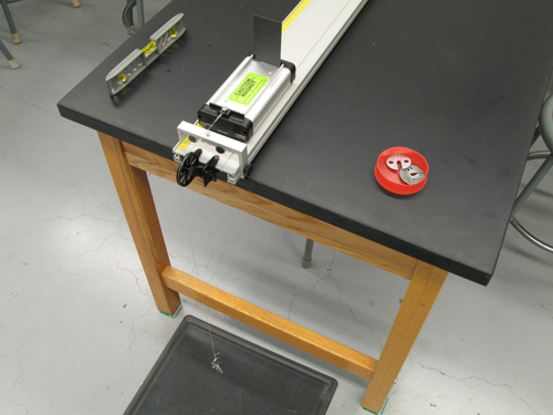
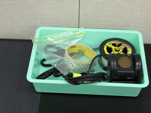
horizontal dynamic track, PASCO pass-cart, motion sensor connected to the Science Workshop Interface, lab stand, balance
Figure 1

Figure 2
Introduction and Theory
Newton's Laws are the essential part of Dynamics—the area of physics that studies the cause of motion experienced by an object. The interaction between objects is measured by a physical quantity—force. A force is a vector quantity, and it can be presented as an arrow. The arrow shows the direction in which the force is being applied, and the length of the arrow shows the magnitude (size) of the force. The two types of forces are contact forces and field forces. Examples of contact forces are friction force, normal force, and tension force. Examples of field forces are gravity force and electromagnetic force. Usually there is more than one force applied to an object. To predict the type of motion an object will experience due to forces acting on it, a net force needs to be calculated. A net force is a vector sum of all the forces that act on the object. Newton's First Law states that an object will be at rest or will maintain constant velocity motion until a nonzero net external force acts on it. In other words, if the vector sum of all the forces applied to an object (or net force) is zero, the object stays at rest or is moving with constant velocity. The system of reference where this fact holds true is called an inertial system of reference. If the forces are not balanced (which means a net force does not equal zero), the object will move with constant acceleration, which will be directly proportional to the net force and inversely proportional to an object's mass. Newton's Second Law of motion can be summarized by the following equation, where ΣF represents a net external force acting on an object, m is the mass of the object moving under the influence of ΣF, and a is the acceleration of that object. ΣF and a are vector quantities while m—mass—is a scalar quantity. If ΣF = 0, then a = 0, and the object moves at constant velocity as stated in Newton's First Law. If the mass is constant, then acceleration is a linear function, or of the net force. After comparing equations (1) and (2), one can see that the slope of this linear graph equals the inverse value of the system mass. In this case, uncertainty in the experimental value of the system's mass can be found using the rules of error propagation for y = xn since slope = m–1. Newton's Third Law establishes the connection between the action-reaction pair of forces. If two objects collide with each other, then the force of the action will be equal to the force of reaction in magnitude but opposite in direction. Note that in this case, the action and reaction forces applied to the different objects cannot balance (cancel) each other even if they are equal in magnitude. In this lab, you will validate the first and second laws using a motion sensor and pass-cart(s) moving along a horizontal aluminum track.Video
View the video below prior to beginning your lab.Procedure
Please print the worksheet for this lab. Answer all the questions on the Lab Worksheet prior to submitting the Inlab in WebAssign.Checkpoint:
Be sure to have your TA sign your lab worksheet, printed Inlab, and all printed graphs after each part is completed. Be sure the data can be seen on the graphs.
Be sure to have your TA sign your lab worksheet, printed Inlab, and all printed graphs after each part is completed. Be sure the data can be seen on the graphs.
Newton's First And Second Law
1
Measure the mass of the cart (M) and the mass of the hanger (m).
2
Open the preset experiment file: Desktop/pirt inst labs/PHY 113/PreSet Up Labs/Newton's Second Law. Answer the first question on the lab worksheet.
Experiment 1
3
Put a PASCO cart on the track. Check that the track is leveled. Pressing the Start button will initiate data recording. It stops automatically after 5 seconds. Make a trial run to check if any adjustments to the motion sensor are needed.
4
Pull the cart along the track as far as possible away from the pulley, but not closer than 15 cm to the motion sensor. Press Start. Give a slight push to the cart to make it move.
Caution:
Stop the car by hand before it bangs into the pulley mount at the end of the track.
Stop the car by hand before it bangs into the pulley mount at the end of the track.
Apply "Linear Fit" to the part of the data that corresponds to when the cart was moving at constant velocity. Record the slope. What physics quantity does the slope of this velocity vs. time graph represent? Describe the motion of the cart and explain the reason for it.
Experiment 2
5
In GA, make columns to enter the values of the hanging mass (kg) and acceleration (m/s2).
6
Arrange four 10.0-g masses on the top of the cart so that they are evenly distributed. Hang another 10.0-g mass on the S-shaped hanger. Again, pull the cart along the track as far as possible away from the pulley, but not closer than 15 cm to the motion sensor. Press Start and release the cart. As before, stop the car by hand before it bangs into the pulley. Apply "Linear Fit" to the part of the data that is not in immediate proximity to the magnetic stopper. Use the slope of the graph to get its acceleration.
7
Repeat the above steps to make four additional runs. For each consecutive run, remove a 10.0-g mass from the cart, then place it on the hanger. No matter how many 10.0-g masses remain on the cart, always try to keep the masses on the cart symmetrically distributed. Record acceleration of the cart for each run.
8
After all data is entered, make a calculated column in GA to find the gravity force applied to the cart. Since the friction force is negligible, the magnitude of the gravity force is equal to the magnitude of the net force applied to the system (cart + hanging weight), although their directions are different. Plot the acceleration of the system vs. the magnitude of the gravity force. Apply "Linear Fit" to this graph. Using the parameters of the regression line of this graph, calculate the experimental mass (mexp) of the system along with its uncertainty. Compare the experimental value of the system's mass (cart + hanger + additional weights) calculated from the slope of the graph to the one measured with the balance.
Experiment 3: Prediction
9
Predict the acceleration of this cart for the force magnitude that is given in the Inlab. Does your data support the mathematical model for Newton's Second Law?


