Linear Motion
Back to TopObjectives
-
•to compare the relationship between position vs. time and velocity vs. time for different types of linear motion
-
•to measure the value of gravitational acceleration g on Earth by the free fall method and compare it to the accepted value
Equipment
battery-powered constant speed cart, masking tape, cardboard, PASCO motion sensor, fan cart, track Spring Semester: small rubber object or whiffle ball, stop watch, 30-m measuring tape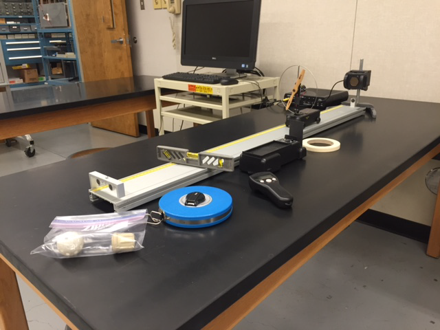
Figure 1: Spring Semester Equipment
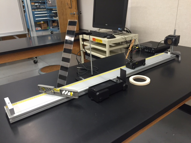
Figure 2: Fall Semester Equipment
Introduction and Theory
Kinematics is the area of physics that studies types of motion without specifying what caused it. The three major types of simple linear motion are constant velocity motion, uniformly accelerated linear motion, and free fall. The basic physics quantities used to describe the motion of an object are: position, distance, displacement, speed, velocity, and acceleration. The description is sufficient if one can specify the location of the object at any specific time. There are a number of ways of representing motion. One of them is to use a motion diagram. Fig. 3 presents a motion diagram of an object moving at constant acceleration. Each dot presents a position of an object registered in an equal time interval.
Figure 3: Motion Diagram for Constant Acceleration
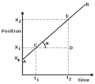
Figure 4: Position vs. Time Plot
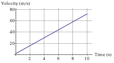
Figure 5: v(t) Graph
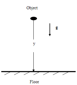
Figure 6
Fig. 7
presents a motion diagram of the free fall motion of the object before it reaches terminal velocity. This diagram has a similar view as the one for the uniformly accelerated motion above. A free-falling object experiences a uniformly accelerated motion until it reaches its terminal velocity.

Figure 7: Motion Diagram for Free Fall
Video
View the video below prior to beginning your lab.Procedure
Please print the worksheet for this lab. Answer all the questions on the Lab Worksheet prior to submitting the Inlab in WebAssign.Checkpoint:
Print only the section of the worksheet that applies to your semester. Be sure to have your TA sign your lab worksheet, printed Inlab, and all printed graphs after each part is completed. Be sure the data can be seen on the graphs.
Print only the section of the worksheet that applies to your semester. Be sure to have your TA sign your lab worksheet, printed Inlab, and all printed graphs after each part is completed. Be sure the data can be seen on the graphs.
Part 1: The cart moves toward the motion sensor at a constant speed.
1
On the lab worksheet, sketch the graphs you expect to be produced by the cart moving toward the motion sensor with constant speed.
2
Turn on the interface. Open the presetup file "Linear Motion" located at Desktop/pirt inst labs/PHY 113/PreSet Up Labs/Linear Motion. Be sure the Start button shows active in the software.
To calibrate the motion sensor: Click Calibrate Sensor, and then click on Motion Sensor. Type "standard distance 1m." Place a 1-m ruler between the sensor and the cart. Remove the ruler and click set the standard distance. You should see 1 m appears in the window on the screen. Close the calibration window.
3
Place the constant speed cart at the opposite end of the track from the motion sensor. Using masking tape, make a mark on the track 20 cm away from the motion sensor. Turn on and hold the cart. Click Start in the Data Studio software and release the cart. Stop the recording when the cart reaches a 20-cm mark.
In a group, discuss what kind of graphs were produced by the motion of the cart. Do they look as you expected them to look? Record the major points of your discussion in the worksheet for this lab.
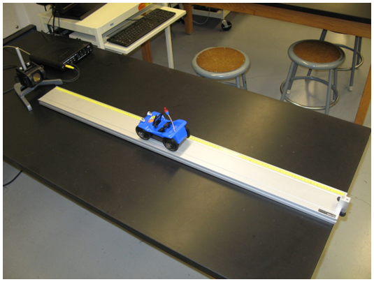
Figure 8
4
You should see on the screen the position vs. time graph and velocity vs. time graph of the cart's run produced by the software. Use the "Autofit" function to resize the graphs.

Figure 9
5
On the position vs. time graph, highlight (drag around with the computer cursor) the part of the plot corresponding to the cart moving along the track with constant speed. Apply "Linear Fit." (Hint: Select "Linear Fit" in the pull-down Fit menu.)

Figure 10
6
Login to your WebAssign account. Open the Linear Motion Inlab and complete Table 1. Complete all of the following questions for "Part 1: Constant Velocity Motion." Take a screenshot of the graphs with the data from "Linear Fit." Paste and save them in a document in DOC format. Upload this file in the Inlab for Part 1.
Part 2: Uniformly Accelerated Motion
1
On the lab worksheet, sketch the graphs you expect to be produced by the sail cart moving away from the motion sensor with constant acceleration.
2
Attach a piece of the cardboard to the side of the fan cart facing the motion sensor. Place the fan cart 20 cm away from the motion sensor and oriented so that it will move away from the motion sensor. Turn on the fan and start the program. Stop recording the data when the cart reaches the other end of the track. Stop the cart.
In a group, discuss what kind of graphs are produced by the motion of the cart. Do they look as you expected them to look? Compare these graphs to the ones received in Part 1. Record the major points of your discussion on the worksheet for this lab.
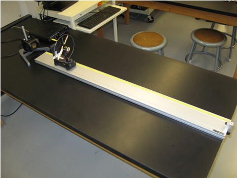
Figure 11
3
On the position vs. time graph, highlight the curved part of the graph corresponding to the cart accelerating along the track. Fit the selected part of the data with a "Quadratic Fit" function.

Figure 12
4
Complete Table 2 in the Linear Motion Inlab in WebAssign. Answer all the following questions for this part of the lab. Take a screenshot of the graphs with the data from "Quadratic Fit." Paste and save them in a document in DOC format. Upload this file in the Inlab for Part 2.
Part 3: Free Fall
Caution:
Depending on the semester you take the lab, you will either do the Free Fall Experiment A. Stairway or B. Photogate.
Depending on the semester you take the lab, you will either do the Free Fall Experiment A. Stairway or B. Photogate.
A. Stairway (Spring Semester)
1
Drop the provided object from the stairway of a building. Make sure that no one is directly below the object when it is dropped. Use a tape measure to determine the height y from which the object is released. Use the stopwatch to measure the time t it takes for the
object to fall down to the ground. These measurements have to be repeated at least 6 times in order to get a reasonable value of t
along with the associated error.
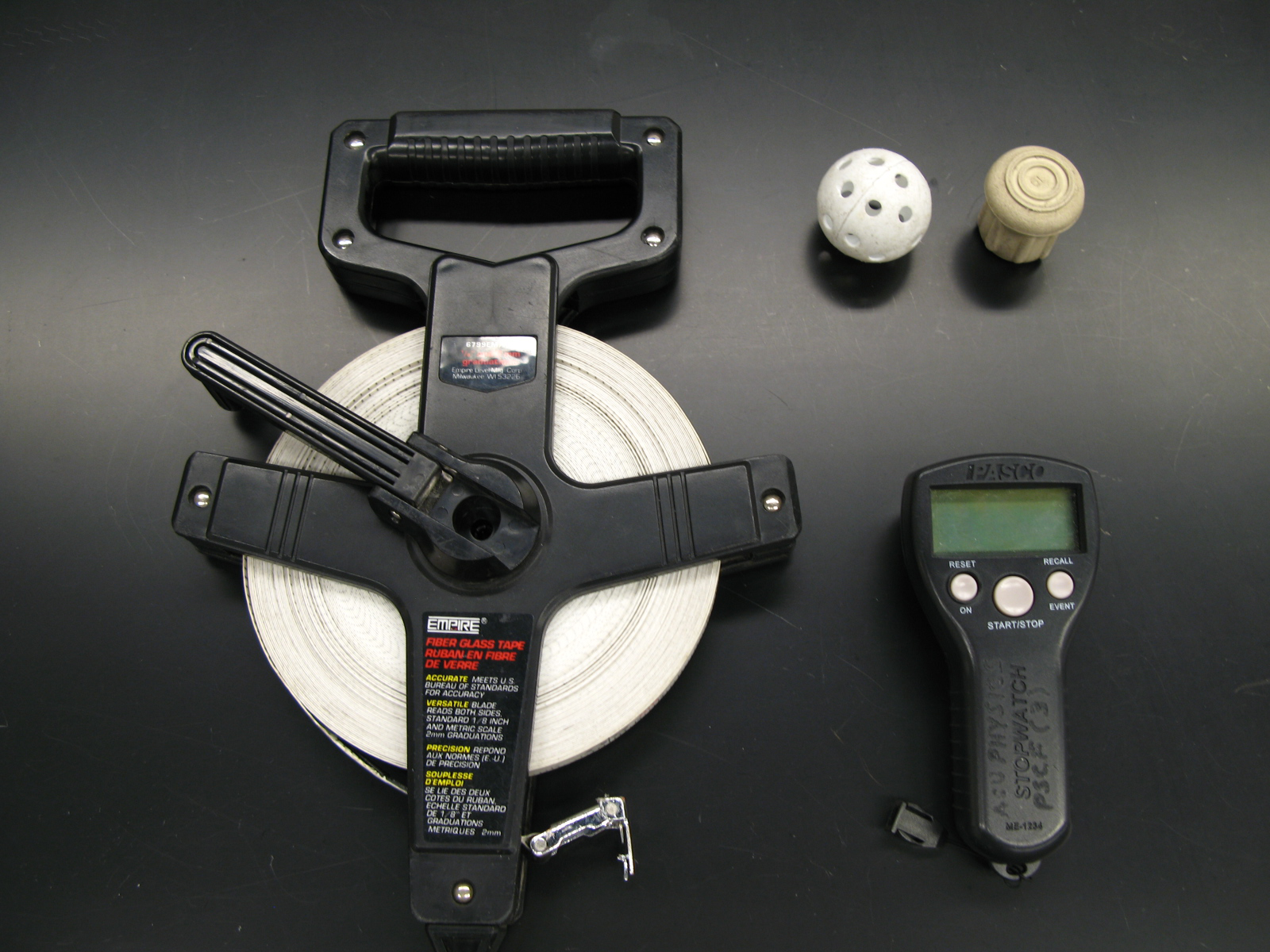
Figure 13
2
Record measurements of the height and time on the lab worksheet. Assume the error in height is 2.0 cm.
3
In GA, enter the values of time. Use "Statistics" to find the mean value of time and standard deviation. Take a screenshot of the statistics graphs with the provided data. Paste and save them in a document in DOC format. Upload this file in the Inlab for Part 3. Using these data, you will evaluate the value of gravitational acceleration g that each object
has experienced, and its uncertainty.
4
Complete Part 3 in the Linear Motion Inlab in WebAssign. Be sure to upload a statistics graph from GA.
Discuss with your group members if the experimental value of g agrees with the expected one. Record the major points of your discussion on the lab worksheet.
B. Photogate (Fall Semester)
1
Turn on the interface and open the pre-set experiment file: Desktop/Labs/PHY 113/PreSetUp Files/Free Fall.
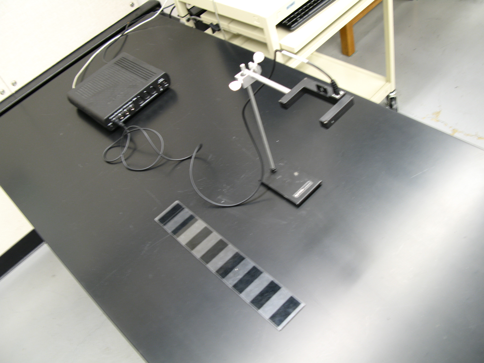
Figure 14
2
Position the stand with a photogate at the edge of the lab table in such a way that you can safely drop the long picket fence all the way through. Bring the rubber or foam pad directly underneath the photogate onto the floor to cushion the landing of the picket fence. Try to catch the picket fence after it passes through the photogate.
3
Press the Start button and carefully drop the picket fence through the photogate. (See Appendix B for more information.) The software stops collecting the data automatically after 5 seconds. Apply "Linear Fit" to your velocity data displayed on the graph to get the acceleration of the falling picket fence. Repeat
this procedure 5 times.
4
In GA, create a new manual column. (Hint: Data → New Manual Column "Gravitational Acceleration") Remember to name it and choose an appropriate unit.
Then, in GA, enter the values of 5 measured accelerations. Use "Statistics" to find the mean value of the experimental g and the standard deviation. Record this and complete all the questions for Part 3 in the Inlab in WebAssign. Take a screenshot of the statistics graphs with the provided data. Paste and save them in a document in DOC format. Upload this file in the Inlab for Part 3.

