
Conservation of Mechanical Energy; Work
Purpose
-
•To study conservation of mechanical energy for a cart moving along an incline.
-
•To observe the scalar nature of energy.
-
•To examine the nonconservative nature of the friction force.
Equipment
- Dynamics Track Simulation
- Pencil
Simulation and Tools
Open the Dynamics Track simulation to do this lab. See the Video Overview.Explore the Apparatus
Open the Dynamics Track. You should be familiar with most of the features of the ramp and cart system from your study of kinematics and dynamics. There are just a few new features that you should familiarize yourself with now.Setting the Initial Velocity, "V0"
Figures 1 and 3 show parts of the control panel beneath the right end of the track. These controls are used to set the initial velocity of the cart as well as the static and kinetic friction between the cart and track. The panel's appearance changes according to the situation.
Figure 1: Initial Velocity Controls
–300 cm/s
to +300 cm/s.
You can change the direction of the velocity by inserting (or deleting) a – sign, or use the "V0" stepper gadget
 to move through the range of positive and negative velocities.
Adjusting the Kinetic and Static Friction, "μK" and "μS"
By default, the cart runs on frictionless wheels. This is indicated by the selected radio button next to "wheels." To allow you to investigate motion with frictional resistance, the wheels can be replaced by a friction pad with variable friction coefficients—kinetic, "μK," and static, "μS." When the unselected radio button
 is clicked, it becomes selected
, and the friction pad controls become active, as shown in Figure 3.
is clicked, it becomes selected
, and the friction pad controls become active, as shown in Figure 3.
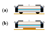
Figure 2: Cart Modes

Figure 3: Initial Velocity Controls
Theory
The kinetic energy of a body is the energy associated with its motion. The potential energy of a physical system is the energy associated with the arrangement of the objects making up the system. This energy is due to the forces among the objects in the system and the work that those forces can do in changing the arrangement of the objects in the system. For example, moving a pair of magnets closer together or farther apart changes the amount of potential energy of the system. In the case of gravitational potential energy for an object near Earth, the energy is due to the force of gravity acting between the objects. If an object at some height above the Earth is allowed to fall to a lower altitude, the loss in potential energy of the system of the Earth and the object would be equal to the work done by the force of gravity. In such a case, the motion of the Earth is negligible, and we usually say that it is the falling object that loses the energy. The change in potential energy of the object is given by where h is measured relative to some arbitrary level where we set h = 0. We define the sum of the kinetic energy and the potential energy of an object (or system) as its total mechanical energy. That is, Note that energy is a scalar quantity, so v is the speed, which is always positive. And h is the height, which can have a negative sign if an object is below the h = 0 reference level. But this does not represent direction. A swinging pendulum is a good example of a system that undergoes a steady change in PE and KE. As the bob rises, its PE increases, and its KE decreases. As it swings back down, the reverse occurs. If there are no forces other than gravity acting, the decrease in one type of energy is exactly matched by the increase in the other. Thus, the total ME remains constant. If the work on the object by nonconservative forces such as friction is zero, the total mechanical energy will remain constant. For such cases, we can say that mechanical energy is conserved.Principle of Conservation of Mechanical Energy:
If Wnc = 0, PE0 + KE0 = PEf + KEf, or ΔPE + ΔKE = 0.
If Wnc = 0, PE0 + KE0 = PEf + KEf, or ΔPE + ΔKE = 0.
Procedure
Please print the worksheet for this lab. You will need this sheet to record your data.
I. Conservation of Mechanical Energy
A. Using Conservation of Mechanical Energy to Predict the Change in Height, Δh, of a Cart Traveling up a Frictionless Ramp and Coming to a Halt
Consider a cart traveling up a frictionless ramp. It will start with a certain initial velocity, v0, and a corresponding amount of initial kinetic energy,| 1 |
| 2 |
 . Click Go and repeat as necessary to observe the following. Note the pink Wx vector (shown as W(x)), which is constant for a given track angle, and always points down the track. This is the component of the weight of the cart acting parallel to the track. As the cart moves, this force does positive or negative work on the cart depending on whether the cart is moving in the direction of the force or opposite it. The green velocity vector varies in magnitude and direction as the cart's kinetic energy changes. So a change in the length of this vector would indicate a ΔKE.
When the cart goes up the ramp, Wx and Δx are in opposite directions, so negative work is done to the cart. Going down the ramp, positive work is done to the cart.
. Click Go and repeat as necessary to observe the following. Note the pink Wx vector (shown as W(x)), which is constant for a given track angle, and always points down the track. This is the component of the weight of the cart acting parallel to the track. As the cart moves, this force does positive or negative work on the cart depending on whether the cart is moving in the direction of the force or opposite it. The green velocity vector varies in magnitude and direction as the cart's kinetic energy changes. So a change in the length of this vector would indicate a ΔKE.
When the cart goes up the ramp, Wx and Δx are in opposite directions, so negative work is done to the cart. Going down the ramp, positive work is done to the cart.
-
•Going up: Work = –|WxΔx|, so ΔKE is also negative, and KE decreases.
-
•Going down: Work = +|WxΔx|, so ΔKE is also positive, and KE increases.
-
•Up then down: Work = –|WxΔx| + |WxΔx| = 0, so ΔKE = 0 (starts and ends at 160 cm/s (speeds, not velocities)).
-
•Use conservation of energy to predict the change in height for a cart given an initial speed at the bottom of the ramp.
-
•Check your prediction by measuring its actual change in height geometrically.
1
Set the ramp angle to any angle from +1° to +5°. Record your chosen ramp angle.
2
Set "Recoil" to 0 and leave it there for all parts of the lab.
3
Turn on the ruler
 .
.
4
By trial and error, find an initial speed that will send the cart to approximately the 170-cm point. Record this as your initial velocity, v0. Note that the cart will start at this initial velocity from a dead start when you click Go. Yes, this would be impossible to do with real physical equipment.
5
Calculate and record KE0 in joules for the 0.250-kg cart. (Careful with units!)
6
Turn on the brake and drag the cart so that the cart mast is at approximately the 20-cm point on the ruler.
7
Turn on the Sensor.
8
Quickly click Go to launch the cart. Turn off the Sensor when the cart returns to the bottom.
Note:
You'll need data from the lab apparatus data table later, so don't use the sensor again until you complete Part IA.
You'll need data from the lab apparatus data table later, so don't use the sensor again until you complete Part IA.
9
Record the cart's final velocity and kinetic energy, vf and KEf, respectively, at the top of the cart's travel. (There are no data required for this. Just think about it.)
10
Using conservation of mechanical energy, calculate and record the cart's predicted change in height, Δh = hf – h0.
11
What Δh would you get if you added 0.250 kg to the cart? Try it to make sure of your answer. (No sensor! See the note above.)
12
That doesn't seem right. It appears that there would be no limit to how much mass could be sent through the same Δh. This would have to "cost" us somehow. Where must this extra energy be coming from?
13
Remove the extra 250 grams from the cart.
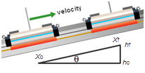
Figure 4: Δh from Trigonometry
14
Scroll through the position data in the right column of the apparatus data table. The initial and final positions of the cart are x0 and xf, respectively, for the trip up the ramp. How can you find x0 and xf from this data? Be careful—the data includes the motion back down the track, which is not what you're looking for.
15
Record x0 and xf.
16
Calculate and record Δh.
17
Calculate the percentage error in your experimental value of Δh. Use your predicted value as the accepted value.
B. The Relationship Between Speed and Kinetic Energy – Proportional Reasoning
Here's your chance to get a better understanding of the nonlinear relationship between speed and kinetic energy. This is something that gives many students trouble.1
Question: Suppose you wanted the cart to start at the same x0 point but rise just half as far vertically, that is, ΔhIA/2. That would mean it would have half the value of ΔPE, which would require just half the initial KE since KEf = 0. You selected a v0 that resulted in a particular ΔhIA. What v0 would you use for ΔhIA/2?
2
We'll find it experimentally first. Add three photogates to the apparatus, just for reference markers. (Click the radio button beside "Photo Gates," then reduce "# Gates" to 3.)
3
Put the first gate at 20 cm, the starting point, x0. Put the third one at the xf you found in Part IA (which is also at the original hf(orig)). Do a test run with your original v0 to make sure that the cart rises to the third photogate (approximately) as it should.
4
For your new target, you need to put the middle gate at the point halfway between the first and third gates. That would be at xmid, which would also be at hmid. Also, xmid should be halfway between x0 and the original xf. (Think about it.)
Calculate and record xmid.
5
You now have a target to shoot at. You first need to experimentally determine the proper v0 to give the cart half of its previous KE. How about v0/2? Try it and see how it works out.
-
aHow'd that work out? Too fast or too slow?
-
bUse trial and error to find your best value for the required initial velocity to just reach xmid. Record v0(mid, expt).
6
Now let's calculate the theoretical initial velocity. Here's the problem and how to think about it.
-
•KE0 =So KE0 is directly proportional to
mv02.1 2 v02,not v0. Sowon't give the cartv0 2
.KE0 2 -
•So halving v0 doesn't halve KE0; halvingv02does!
-
•If you halvev02,you will also halve
mv02.1 2 
m1 2 
v02 2 

-
-
•So if v0(orig) equals your v0 from Part IA, what dov0(orig)2, v0(mid)2 =and v0(mid, theo) equal?
,v0(orig)2 2
7
The proof is in the testing. Give it a try and see if you need further head scratching. (You may need to round to an integer v0.)
II. Work by Friction
As the cart traveled up the ramp in Part IA, gravity did an amount of work equal to –WxΔx on the cart. If the cart is released, on the way back down, gravity would do an amount of work equal to +WxΔx. The total work for the round trip would be zero. That is,−Wx Δx + (+WxΔx) = 0
for the round trip. That's the nature of a conservative force. When work is done in moving an object against such a force, an equal amount of work is done by the force when the object is allowed to return to its starting point. It's as if our work is somehow "stored up" until we need it back.
Of course, most of the time, mechanical energy is not conserved. As you swim across a pool, the water exerts a backward force against you. If you stop and tread water at the other side of the pool, the water will not return the favor (energy) by pushing you back to where you started!
These forces that do a nonzero amount of work when an object is moved around a closed loop are called nonconservative forces. A force like a wind that acts to increase the energy of a sailboat does net positive work. Likewise, a force like friction that removes energy from a system does net negative work. In either case, we can say
where Wnc is the total work done by all nonconservative forces acting. The value of Wnc can be either positive or negative. So it can increase or decrease the energy of an object.
In this part of the lab, we'll look at the negative work done by friction. We'll use a level track and observe the decrease in velocity of the cart when friction is acting. Figure 5 shows the set-up. You won't see the vectors while the car is sitting still. (Two figures were merged to create this figure, and the ruler was dragged way up out of the way.) Notice the decreasing velocity to the right and the constant force to the left (Fnet ≡ Ffriction). There is one force acting, and it is friction.
Note the boxes with the elapsed time, eT, and the time interval, dT, for the 10-cm-wide purple card to pass through the gate. You'll use dT as explained below.
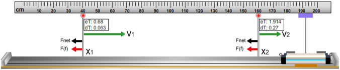
Figure 5: Elapsed Time, eT, and Time Interval, dT

Figure 6: the Measurement of dT
dT1
and dT2,
for the card to pass through a given photogate. These are actually average velocities, Δx/Δt,
but the average velocity is approximately equal to the instantaneous velocity at the midpoint.
1
Set up two photogates as shown above at x1 = 40 cm and x2 = 160 cm.
2
Set "Card Width" to 10 cm.
3
Position the cart at x = 10 cm and set "V0" to 200 cm/s.
4
Turn on the friction pad and set "μK" to 0.10.
5
Click the Take Gate Data button.
6
Click Go.
7
Click the Stop Gate Data button after the cart stops moving.
8
Record your data.
- Δx: distance between gates, distance traveled while work is done by friction, in m
- μk: the known kinetic friction coefficient, no units
- m: the mass of the cart, in kg
- dT1: time to pass through first gate, in s
- dT2: time to pass through second gate, in s
- v1: average speed through first gate (card width/dT), in m/s
- v2: average speed through second gate, in m/s
Note:
Sometimes the dT values are a bit iffy. You may find that one of the dT values is negative. Also, dT2 should be almost twice dT1. Please try again if you see any suspicious data. And be sure to note that you're recording dT, not eT.
Sometimes the dT values are a bit iffy. You may find that one of the dT values is negative. Also, dT2 should be almost twice dT1. Please try again if you see any suspicious data. And be sure to note that you're recording dT, not eT.
9
Calculate your experimental value for μk(expt).
10
Calculate the percentage error in your experimental μk(expt). Use the theoretical value as the accepted value.