
Standing Waves in an Air Column
Purpose
-
•To observe resonance of sound waves in an air column open at one end and closed at the other.
-
•To determine the speed of sound in air and the effect of the air temperature on that speed.
-
•To examine the reflection of sound waves at the closed and open ends of a tube.
-
•To study the effect of the tube length on the resonance frequencies produced.
Equipment
- Virtual Sound Waves simulation
- VPL Grapher
- Pencil
Simulation and Tools
Open the Sound Waves simulation to do this lab. You will need to use the VPL Grapher to complete this lab.Explore the Apparatus/Theory
Use Figure 1 as a reference to identify various parts of the apparatus.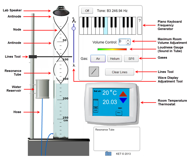
Figure 1
Caution:
If at any time you hear a sound that's too loud, click the Off button at the top of the screen. Be sure to get assistance if you have trouble with this. You don't want to damage your hearing. Also, be careful with headphones. When you first turn on the sound, be sure to have your headphones away from your ears. Once you've determined that the sound seems OK, you can carefully put your headphones on. If you can't lower the headphone volume adequately, you should use speakers instead. It would be better to use just the Loudness Gauge rather than damaging your hearing.
If at any time you hear a sound that's too loud, click the Off button at the top of the screen. Be sure to get assistance if you have trouble with this. You don't want to damage your hearing. Also, be careful with headphones. When you first turn on the sound, be sure to have your headphones away from your ears. Once you've determined that the sound seems OK, you can carefully put your headphones on. If you can't lower the headphone volume adequately, you should use speakers instead. It would be better to use just the Loudness Gauge rather than damaging your hearing.
You need to adjust your computer's system sound level first. This is not set within the lab environment. It's set using your computer's controls. Seek assistance if necessary.
Adjust your computer's system sound level to
- its lowest nonzero setting for headphones.
- near the middle of the range for speakers.
-
•If you use headphones or external speakers to listen to audio, plug them in.
-
•Drag the water reservoir all the way to the top.
-
•Set the room volume setting at 5 in the lab control panel.
-
•Play the "C4" sound frequency on the piano. It's near the middle. You should see the speaker at the top start to vibrate, but you should hear little, if any, sound.
-
•The Loudness Gauge should look something like this:
 . This represents the tube volume.
-
•Adjust the volume on your computer until you can just hear a quiet sound. You're hearing middle C. It doesn't sound like that note as played on any musical instrument since there are no overtones present. It's just a pure, single-frequency sound. As you can see from the display, the C4 note has a frequency of 261.63 Hz. A piano typically has eight octaves. Thus, it has eight C's. C4 is the fourth one from the bottom.
-
•Quickly drag the reservoir until the water level is at about 50 cm. You'll hear the room volume rise and then fall as the water level passes approximately 17 cm. If that peak sound was uncomfortably loud, you need to reduce the computer system volume somewhat and try again. If it was not loud enough, try adjusting the room volume setting in the lab control panel. If necessary, you can adjust your computer system volume.
-
•Continue raising and lowering the water level in this way until you get the volume adjusted to a comfortable level. The target is to be able to hear the sound faintly when the water is at the top and the Loudness Gauge looks like the figure above, while also hearing a louder but comfortable maximum loudness when the water is at about 17 cm.
-
•There's no need to have the room sound on when you're not adjusting the water levels or making readings. It does tend to get annoying very quickly. You can set the room "Volume Control" to 0 to turn off the room sound at any time. The speaker above the tube will continue to play, and there will still be sound in the tube. You just won't hear it. Is that clear? The "Volume Control" controls what you hear—the room sound. The volume of the speaker over the tube will never change unless you turn it Off. Surprisingly, the sound in the tube, the tube volume, will change according to how we adjust various settings in the apparatus.
-
•The Loudness Gauge measures the actual tube volume. When this volume is at its maximum, the gauge will look like this:
 . You'll frequently need to adjust the apparatus in some way to produce the loudest possible sound in the tube. Of course, when the tube volume is loud, the room volume will be, too.
Resonance of Sound in an Air Column
Make sure that you have air in the room (green background). Set the air temperature to 0°C. Drag the reservoir to its highest position and play C4. At any instant, the sound you're hearing was emitted just a fraction of a second before you hear it. Sounds produced a bit earlier have already reached you and jiggled your eardrums. Sounds produced a bit later have yet to reach you. Thus, you're hearing the sound produced at a certain earlier instant. Actually, you're hearing only a small part of that sound since the sound moves off in all directions, dropping off in intensity as it propagates in three dimensions. Now adjust the water level to about 17 cm. The volume reaches a maximum at about that point. So where's all that sound coming from? Actually, it's more like when. (More on this in a moment.) This would be a good time to adjust the "Volume Control" to zero! Drag the wave display adjustment slider until the wave display behind the water looks something like Figure 2.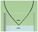
Figure 2
The boundary conditions for standing waves in a closed air column are that an antinode exists at the open end and a node exists at the closed end.
The amplitude of the longitudinal sound wave and corresponding transverse wave displayed is largest where the air has its greatest motion and lowest pressure—an antinode.
The amplitude is smallest where the air has its least motion and greatest pressure—a node.
 |
| 1 |
| 4 |
 |
Procedure
Please print the worksheet for this lab. You will need this sheet to record your data.
I. Finding the Wavelength and Wave Speed from the Spacing of Nodes
1
We'll continue with the same conditions—room thermostat set to 0°C, air in the tube, C4 selected, and the wave display set for a node at about 17 cm as in Figure 2. Turn the volume on so you can hear the sound. Drag the reservoir as far down as it will go. As the air column lengthens, you should hear three more pulses of maximum loudness. Each of these indicates air column lengths that satisfy our two boundary conditions. That is, they indicate additional nodes. See Figure 3.
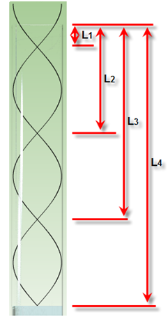
Figure 3
2
The transverse wave revealed as the water falls provides a good record of these nodal points. But you'll probably need to do some adjustments. The loudness of the sound doesn't go from zero to its maximum at a point but rather over a range of several centimeters. So it's tricky to estimate just where the nodes are. By watching the Loudness Gauge while making fine adjustments to the transverse wave display, you should be able to make each of its four nodal points correspond nicely to the corresponding points of maximum loudness. You'll see that setting the bottom-most node yields the most precise results. Go ahead and do that fine tuning.
3
Using Table 1,
-
•record your values for lengths L1 and L4.
-
•calculate λc and record it as your wavelength value, λ.
-
•calculate the velocity of sound in air at 0°C using equation 1v = λf,with λ.
-
•calculate the percentage error between your experimental value for the velocity of sound in air at 0°C and the accepted value for the speed of sound at 0°C of 331.5 m/s.
II. The Effect of Air Temperature on the Speed of Sound
As you've learned earlier in the course, the volume occupied by a given mass of gas, and hence its density, varies with temperature. If the density of the gas occupying our tube changes with temperature, perhaps its velocity does too.1
Reset the conditions in the tube again as before—room thermostat set to 0°C, air in the tube, C4 selected. Adjust the water level to L4 so that you're hearing the amplified sound in the tube. Use the lines tool to put a marker at the L4 (0°C) position.
Record the value of L4 (0°C).
2
If you have the room volume set to zero, adjust it to an audible level for the following. Increase the air temperature to its maximum value of 40°C. Listen for changes in the loudness. OK, you can reset the room volume if you like.
As you increased the temperature, what happened to the loudness of the sound?
3
Adjust the water level up or down until you find the new location of the fourth node. It could be further up the tube or further down. You'll have to figure out which one is the new L4 position.
-
aRecord the value of L4 (40°C).
-
bHas the wavelength of the sound increased or decreased?
4
Given that there is a change in wavelength, this must mean that either the speed or the frequency has changed, or possibly both. You probably didn't notice any change in the frequency, and this is reasonable given that the frequency of the sound is determined by the frequency of vibration of the speaker. So it's the velocity that must have changed.
5
Based on equation 1v = λf,
, has the speed of sound increased or decreased with this increase in temperature? Explain your reasoning.
6
Let's determine the relationship between the speed of sound in air and the temperature of the air. We again need to determine the wavelength experimentally and then calculate the wave speed using equation 1 for each temperature setting. Just as before, we'll find λc from equation 4λc =
(L4 − L1)
. Calculate and record this as your wavelength, λ, for each temperature in Table 2.
Use Table 2 to find the velocity at each of the five temperatures given. We're looking for very small changes, particularly in the L1 value. Patience is a virtue.
| 2 |
| 3 |
7
You should have found that the speed increased with temperature as predicted. To find the relationship, plot velocity vs. temperature. We'll use Celsius degrees, °C, for our temperature units. You should find a fairly linear graph with Grapher. Use manual mode and start both axes at 0. (Be sure to click in an empty cell after entering the last data point. Otherwise, it won't show up.)
Sketch your graph on the grid in Figure 4. Take a Screenshot
 of your graph and upload it as "soundwaves_vt".
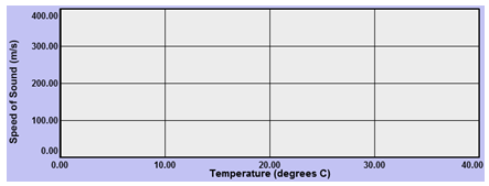
Figure 4
8
Write your equation in y = mx + b
format.
9
Using the accepted values (for this apparatus) for the slope and y-intercept gives the equation
This is an empirical equation that works fairly well for a limited range of temperatures. To see how well your results compare to these accepted values, calculate the percentage error for your slope and for your y-intercept.
III. Determining the End Correction for the Tube
We found that our sound wave resonated in an air column that extended somewhat beyond the top of the tube. We now want to determine the length of this extra column of air, the "end correction." This end correction is represented by the dark rectangle at the top of Figure 5.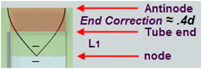
Figure 5
1
Determine the experimental value of the end correction.
2
By careful analysis, the resonating column of air is found to extend approximately 0.4 × diameter of tube. We will use this as the accepted value. The tube's diameter is 0.38 m.
3
Determine the theoretical value of the end correction, 0.4 × diameter of tube.
4
Calculate the percentage error between the experimental and theoretical values for the end correction.
Note that this end correction is considered a part of the standing wave even though it is outside the physical tube. Be sure to include it in any calculations involving the effective length of the resonating air column.
IV. The Effect of Air Column Length on Resonance Frequencies; Musical Instruments
Let's finish up with something a bit more musical! If there came a time when we needed to leave this planet to set up our civilization elsewhere, we would need to build a pretty large musical ark to carry all the different wind instruments that people, animals, and inanimate nature have invented. They all work based on the same basic principles as our glass tube, but they are way more complex. And even the performer is part of the instrument. If you'd like to know more, please check out "The Physics of Music" by David Lapp. With the exception of a few instruments such as the bugle, all wind instruments play a fundamental frequency along with other higher pitches that can be produced by changing the effective length of the resonating air column. So where do the notes come from? A wind source such as your lungs or an actual natural wind provides a supply of moving air, which passes into or, in the case of whistling, out of the instrument. The airflow is interrupted by some sort of "reed" that interrupts the flow of the air at a frequency controlled by the dimensions of the instrument. We want to investigate how the resonance frequency is related to the length of the resonating air column. The dimensions of the tube as well as the placement of openings along its length determine the frequency of the wave that will resonate in the tube and influence the frequency of the reed.1
To make life more comfortable for our musicians, we'll use a temperature of 20°C for this section. We'll also use 342.7 m/s and 0.15 m
for the speed of sound and end correction, respectively.
2
With no tone playing (click OFF), drag the water reservoir all the way to the top.
3
Drag the wave display slider all the way to the top.
4
Play C3. It should be barely audible, if at all.
5
Slowly drag the reservoir downward until the maximum volume is heard for the first time.
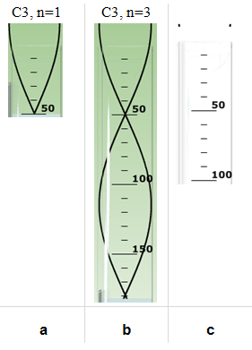
Figure 6
6
Adjust the wave display to match Figure 6a.
7
Carefully drag the reservoir downward until the sound becomes quiet and then reaches its second maximum.
8
Adjust the wave display, if necessary, to match Figure 6b.
n = 1, 3, 5, ..., n =
the number of quarter waves that will exactly fit into the length, L.
Ex. For Figure 6a, we have a quarter wavelength in the air column, where
which is pretty close.
Our λ1 looks about right given the distance—about 1.32 m—we see between the two nodes in Figure 6b. And our f1 is pretty close to the 130.81 Hz note we played.
n = 1,
v = 342.7 m/s,
and L = 0.51 m + 0.15 m = 0.66 m.
We'll use these values for v (342.7 m/s)
and the end correction (0.15 m) in this development instead of your experimental values.
From equations 6 and 7,
λ1 =
=
= 2.64 m
| 4L |
| n |
| 4 × 0.66 m |
| 1 |
f1 =
=
= 129.81 Hz,
| nv |
| 4L |
| 1 × 342.7 m/s |
| 4 × 0.66 m |
λn =
and 7| 4L |
| n |
fn =
,
predict what wavelengths and frequencies will be needed for resonance just based on the wave speed and the length of the air column!
Also notice that in equation 6, the "n" term allows only a quarter wavelength air column, a three-quarter wavelength air column, etc. This matches our boundary conditions. Figures 6a and 6b both contain waves of identical frequency and wavelength. A larger L value will only produce standing waves if some other odd number of quarter wavelengths will fit.
But what will happen if we try a different frequency with the same initial length, | nv |
| 4L |
L = 0.66 m?
9
Reset the apparatus with C3 and L = λ/4
as in Figure 6a.
10
Click D3, which is the next white key to the right. No resonance. And the result is the same for E3 and F3.
11
Repeat with every key until you find another note that produces strong resonance.
12
Record the second frequency producing resonance in an air column of length 0.66 m.
13
Don't move the wave display slider yet. Instead, in Figure 6c, draw the standing wave, with n = 3,
that you think is present in this tube with this new higher frequency. The tops of the waves are provided to get you started. Think about how this new resonant frequency compares to C3. Is its frequency higher or lower than C3? Would its wavelength be longer or shorter? Look back at the discussion of boundary conditions in the exploration section. How could the G4 tone fit within the 66-cm length and still meet the boundary conditions?
14
Adjust the wave display slider to match your figure. You can then see if you were correct by moving the water reservoir up and down. You should see that you'll get resonance at both nodes! Make any corrections necessary to Figure 6c.
15
Take a Screenshot
of the upper end of the tube and upload it as "soundwaves_Figure6c".
16
How many quarters of C3's wavelength fit in this 0.66-m "tube"?
17
What did we find above for C3's wavelength?
18
How many quarters of G4's wavelength fit in this 0.66-m "tube"?
19
Using equation 6λn =
, determine G4's wavelength.
| 4L |
| n |
20
Show your theoretical calculations of G4's wavelength and frequency using equations 6λn =
and 7| 4L |
| n |
fn =
,
.
| nv |
| 4L |
21
What do the two values for n in #16 and #18 tell you about the two frequencies? You can find out by considering the fact that for a constant velocity, λC3fC3 = λG4fG4.
22
Show your calculations of the ratio of | fG4 |
| fC3 |
That is,
-
1st harmonic: C3 f1 = 130.81 Hz fundamental frequency 2nd harmonic: C4 f2 = 261.63 Hz 3rd harmonic: G4 f3 = 392 Hz 1st overtone.
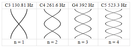
Figure 7: Harmonics 1–4 for an open tube
Figure 7. The equations matching equations 6
λn =
and 7| 4L |
| n |
fn =
,
for an open tube are slightly different.
where | nv |
| 4L |
n = 1, 2, 3, ..., n =
the number of half waves that will exactly fit into the length, L.
For a given note, would the dimensions of these tubes be the same as with our closed tubes? We'll leave that for you to calculate. Unfortunately, you can't test it with our apparatus.
This difference in the harmonics that can be played by an instrument is one of the ways in which we distinguish between them when we hear them. These distinguishing characteristics of the sounds of different "instruments" is known as their timber (TAM-ber or TIM-ber) or tone quality. It's actually more subtle than just the harmonics they can play. Otherwise, all closed tubes of a given length would sound the same.
If you listened to an orchestra's wind section all playing together, you might not know the names of the different instruments, but you could certainly distinguish one from another. This is due to the power of the sounds of the different harmonics that each produces. For example, a typical open flute plays the first and third harmonics very strongly, but the second is not so strong. After the third harmonic, the power gradually diminishes with a few strong harmonics here and there.
A clarinet characteristically plays the first several odd harmonics at about even power, but the even harmonics are produced at somewhat less power. A bassoon typically rises in power from the first up to the fourth harmonic, stays steady, and then begins to diminish in power.
The player of the instrument also plays some role in the tone quality. And speaking of the human input, you've probably observed that when you get a phone call on a not-so-great phone, it's hard to tell who's calling even if it's a close friend. That's because a better quality phone is one that can accurately reproduce the sound spectrum of the caller. And this works for both ends. A call will only be clear if both phones have good fidelity. In ancient times, a.k.a. the 50s and 60s, "records" often had the words "Hi Fidelity" prominently printed on their covers. And they sounded best if you played them on a good "Hi Fi."
In a less musical case, if someone drops an object out of your view, you could very likely tell them whether it was, say, a screwdriver, a wrench, or a teaspoon. And if it was a wrench, you could probably suggest approximately how long it was.
Finally, why is the buzzing sound that we're working with in this lab so unpleasant? I was puzzling on this and momentarily considered the possibility that a single frequency is not very common given that most sounds that we hear involve something that can produce a range of frequencies. Then it hit me. Bees, mosquitos, electric saws, dentist drills... Hmm.
Beware the buzz!